
Predicting Spectral Information for Self-Supervised Signal Classification
Proceedings of the Thirty-Fourth International Joint Conference on Artificial Intelligence. Main Track. Pages 6758-6766.
https://doi.org/10.24963/ijcai.2025/752
Keywords
- Machine Learning: ML: Time series and data streams
- Machine Learning: ML: Classification
- Machine Learning: ML: Self-supervised Learning
- Machine Learning: ML: Representation learning
Abstract
Deep learning methods have demonstrated remarkable performance across various communication signal processing tasks. However, most signal classification methods require a substantial amount of labeled samples for training, posing significant challenges in the field of communication signals, as labeling necessitates expert knowledge. This paper proposes a novel self-supervised signal classification method called Spectral-Guided Self-Supervised Signal Classification (SGSSC). Specifically, to leverage frequency-domain information with modulation semantics as prior knowledge for the model, we design a previously unexplored pretext task tailored to the format of signal data. This task involves predicting spectral information from masked time-domain signals, enabling the model to learn implicit signal features through cross-domain pattern transformation. Furthermore, the pretext task in the SGSSC method is relevant to the downstream classification task, and using traditional fine-tuning strategies on the downstream task may lead to the loss of certain features associated with the pretext task. Therefore, we propose an attention mechanism-based fine-tuning strategy that adaptively integrates pre-trained features from different levels. Extensive experimental results validate the superiority of the SGSSC method. For instance, when the proportion of labeled samples is only 0.5%, our method achieves an average improvement of 2.3% in downstream classification tasks compared to the best-performing self-supervised training strategies.
- [Andrzejak et al., 2001] Ralph G Andrzejak, Klaus Lehn- ertz, Florian Mormann, Christoph Rieke, Peter David, and Christian E Elger. Indications of nonlinear deterministic and finite-dimensional structures in time series of brain electrical activity: Dependence on recording region and brain state. Physical Review E, 64(6):061907, 2001.
- [Anguita et al., 2013] Davide Anguita, Alessandro Ghio, Luca Oneto, Xavier Parra, Jorge Luis Reyes-Ortiz, et al. A public domain dataset for human activity recognition using smartphones. In Esann, volume 3, page 3, 2013.
- [Cai et al., 2022] Jingjing Cai, Fengming Gan, Xianghai Cao, and Wei Liu. Signal modulation classification based on the transformer network. IEEE Transactions on Cog- nitive Communications and Networking, 8(3):1348-1357, 2022.
- [Caron et al., 2020a] Mathilde Caron, Ishan Misra, Julien Mairal, Priya Goyal, Piotr Bojanowski, and Armand Joulin. Unsupervised learning of visual features by con- trasting cluster assignments. In H. Larochelle, M. Ranzato, R. Hadsell, M.F. Balcan, and H. Lin, editors, Advances in Neural Information Processing Systems, volume 33, pages 9912-9924.
- Curran Associates, Inc., 2020.
- [Caron et al., 2020b] Mathilde Caron, Ishan Misra, Julien Mairal, Priya Goyal, Piotr Bojanowski, and Armand Joulin. Unsupervised learning of visual features by con- trasting cluster assignments. Advances in neural informa- tion processing systems, 33:9912-9924, 2020.
- [Chen and He, 2021] Xinlei Chen and Kaiming He. Explor- ing simple siamese representation learning. In Proceed- ings of the IEEE/CVF Conference on Computer Vision and Pattern Recognition (CVPR), pages 15750-15758, June 2021.
- [Chen et al., 2020a] Ting Chen, Simon Kornblith, Moham- mad Norouzi, and Geoffrey Hinton. A simple frame- work for contrastive learning of visual representations. In Hal Daumé III and Aarti Singh, editors, Proceedings of the 37th International Conference on Machine Learning, vol- ume 119 of Proceedings of Machine Learning Research, pages 1597-1607. PMLR, 13-18 Jul 2020.
- [Chen et al., 2020b] Ting Chen, Simon Kornblith, Moham- mad Norouzi, and Geoffrey Hinton. A simple framework for contrastive learning of visual representations. In In- ternational conference on machine learning, pages 1597- 1607. PMLR, 2020.
- [Chuang et al., 2020] Ching-Yao Chuang, Joshua Robinson, Yen-Chen Lin, Antonio Torralba, and Stefanie Jegelka. Debiased contrastive learning. Advances in neural infor- mation processing systems, 33:8765-8775, 2020.
- [Dau et al., 2019] Hoang Anh Dau, Anthony Bagnall, Kaveh Kamgar, Chin-Chia Michael Yeh, Yan Zhu, Shaghayegh Gharghabi, Chotirat Ann Ratanamahatana, and Eamonn Keogh. The ucr time series archive. IEEE/CAA Journal of Automatica Sinica, 6(6):1293-1305, 2019.
- [Doersch et al., 2015] Carl Doersch, Abhinav Gupta, and Alexei A Efros. Unsupervised visual representation learn- ing by context prediction. In Proceedings of the IEEE in- ternational conference on computer vision, pages 1422- 1430, 2015.
- [Dosovitskiy et al., 2020] Alexey Dosovitskiy, Lucas Beyer, Alexander Kolesnikov, Dirk Weissenborn, Xiaohua Zhai, Thomas Unterthiner, Mostafa Dehghani, Matthias Min- derer, Georg Heigold, Sylvain Gelly, et al. An image is worth 16x16 words: Transformers for image recognition at scale. arXiv preprint arXiv:2010.11929, 2020.
- [Dwibedi et al., 2021] Debidatta Dwibedi, Yusuf Aytar, Jonathan Tompson, Pierre Sermanet, and Andrew Zisser- man. With a little help from my friends: Nearest-neighbor contrastive learning of visual representations. In Proceed- ings of the IEEE/CVF International Conference on Com- puter Vision, pages 9588-9597, 2021.
- [Eldele et al., 2023] Emadeldeen Eldele, Mohamed Ragab, Zhenghua Chen, Min Wu, Chee-Keong Kwoh, Xiaoli Li, and Cuntai Guan. Self-supervised contrastive represen- tation learning for semi-supervised time-series classifica- tion. IEEE Transactions on Pattern Analysis and Machine Intelligence, 2023.
- [Emam et al., 2020] Ayman Emam, M Shalaby, Mo- hamed Atta Aboelazm, Hossam E Abou Bakr, and Hany AA Mansour. A comparative study between cnn, lstm, and cldnn models in the context of radio modulation classification. In 2020 12th International Conference on Electrical Engineering (ICEENG), pages 190-195. IEEE, 2020.
- [Fonseca Guerra et al., 1998] C Fonseca Guerra, JG Sni- jders, G t Te Velde, and E Jan Baerends. Towards an order- n dft method. Theoretical Chemistry Accounts, 99:391- 403, 1998.
- [Franceschi et al., 2019] Jean-Yves Franceschi, Aymeric Dieuleveut, and Martin Jaggi. Unsupervised scalable representation learning for multivariate time series. In H. Wallach, H. Larochelle, A. Beygelzimer, F. d'Alché- Buc, E. Fox, and R. Garnett, editors, Advances in Neural Information Processing Systems, volume 32.
- Curran Associates, Inc., 2019.
- [Hamidi-Rad and Jain, 2021] Shahab Hamidi-Rad and Swayambhoo Jain. Mcformer: A transformer based deep neural network for automatic modulation classification. In 2021 IEEE Global Communications Conference (GLOBECOM), pages 1-6, 2021.
- [He et al., 2020] Kaiming He, Haoqi Fan, Yuxin Wu, Sain- ing Xie, and Ross Girshick. Momentum contrast for un- supervised visual representation learning. In Proceedings of the IEEE/CVF Conference on Computer Vision and Pat- tern Recognition (CVPR), June 2020.
- [He et al., 2022] Kaiming He, Xinlei Chen, Saining Xie, Yanghao Li, Piotr Dollár, and Ross Girshick. Masked au- toencoders are scalable vision learners. In Proceedings of the IEEE/CVF Conference on Computer Vision and Pat- tern Recognition (CVPR), pages 16000-16009, June 2022.
- [Hermawan et al., 2020] Ade Pitra Hermawan, Rizki Rivai Ginanjar, Dong-Seong Kim, and Jae-Min Lee. Cnn-based automatic modulation classification for beyond 5g com- munications. IEEE Communications Letters, 24(5):1038- 1041, 2020.
- [Hong et al., 2017] Dehua Hong, Zilong Zhang, and Xi- aodong Xu. Automatic modulation classification using re- current neural networks. In 2017 3rd IEEE International Conference on Computer and Communications (ICCC), pages 695-700, 2017.
- [Huang et al., 2021] Sai Huang, Chunsheng Lin, Wenjun Xu, Yue Gao, Zhiyong Feng, and Fusheng Zhu. Identifica- tion of active attacks in internet of things: Joint model-and data-driven automatic modulation classification approach. IEEE Internet of Things Journal, 8(3):2051-2065, 2021.
- [Huynh-The et al., 2020] Thien Huynh-The, Cam-Hao Hua, Quoc-Viet Pham, and Dong-Seong Kim. Mcnet: An ef- ficient cnn architecture for robust automatic modulation classification. IEEE Communications Letters, 24(4):811- 815, 2020.
- [Jing and Tian, 2020] Longlong Jing and Yingli Tian. Self- supervised visual feature learning with deep neural net- works: A survey. IEEE transactions on pattern analysis and machine intelligence, 43(11):4037-4058, 2020.
- [Katsaggelos et al., 1993] A.K. Katsaggelos, K.T. Lay, and N.P. Galatsanos. A general framework for frequency do- main multi-channel signal processing. IEEE Transactions on Image Processing, 2(3):417-420, 1993.
- [Kong et al., 2023] Weisi Kong, Xun Jiao, Yuhua Xu, Bolin Zhang, and Qinghai Yang. A transformer-based con- trastive semi-supervised learning framework for automatic modulation recognition. IEEE Transactions on Cognitive Communications and Networking, 9(4):950-962, 2023.
- [Liu and Chen, 2024] Jiexi Liu and Songcan Chen. Timesurl: Self-supervised contrastive learning for universal time series representation learning. In Proceed- ings of the AAAI Conference on Artificial Intelligence, volume 38, pages 13918-13926, 2024.
- [Luo et al., 2023] Dongsheng Luo, Wei Cheng, Yingheng Wang, Dongkuan Xu, Jingchao Ni, Wenchao Yu, Xuchao Zhang, Yanchi Liu, Yuncong Chen, Haifeng Chen, et al. Time series contrastive learning with information-aware augmentations. In Proceedings of the AAAI Conference on Artificial Intelligence, volume 37, pages 4534-4542, 2023.
- [Noroozi and Favaro, 2016] Mehdi Noroozi and Paolo Favaro. Unsupervised learning of visual representations by solving jigsaw puzzles. In Bastian Leibe, Jiri Matas, Nicu Sebe, and Max Welling, editors, Computer Vision -ECCV 2016, pages 69-84, Cham, 2016. Springer International Publishing.
- [Oord et al., 2018] Aaron van den Oord, Yazhe Li, and Oriol Vinyals. Representation learning with contrastive predic- tive coding. arXiv preprint arXiv:1807.03748, 2018.
- [O'shea and West, 2016] Timothy J O'shea and Nathan West. Radio machine learning dataset generation with gnu radio. In Proceedings of the GNU radio conference, vol- ume 1, 2016.
- [O'Shea et al., 2016] Timothy J O'Shea, Johnathan Corgan, and T Charles Clancy. Convolutional radio modulation recognition networks. In Engineering Applications of Neural Networks: 17th International Conference, EANN 2016, Aberdeen, UK, September 2-5, 2016, Proceedings 17, pages 213-226. Springer, 2016.
- [Pathak et al., 2016] Deepak Pathak, Philipp Krahenbuhl, Jeff Donahue, Trevor Darrell, and Alexei A. Efros. Con- text encoders: Feature learning by inpainting. In Proceed- ings of the IEEE Conference on Computer Vision and Pat- tern Recognition (CVPR), June 2016.
- [Sarkar and Etemad, 2020] Pritam Sarkar and Ali Etemad. Self-supervised ecg representation learning for emotion recognition. IEEE Transactions on Affective Computing, 13(3):1541-1554, 2020.
- [Xu et al., 2011] Jefferson L. Xu, Wei Su, and Mengchu Zhou. Likelihood-ratio approaches to automatic mod- ulation classification. IEEE Transactions on Systems, Man, and Cybernetics, Part C (Applications and Reviews), 41(4):455-469, 2011.
- [Yakkati et al., 2021] Rajesh Reddy Yakkati, Rakesh Reddy Yakkati, Rajesh Kumar Tripathy, and Linga Reddy Cenkeramaddi. Radio frequency spectrum sensing by au- tomatic modulation classification in cognitive radio sys- tem using multiscale deep cnn. IEEE sensors journal, 22(1):926-938, 2021.
- [Zeng et al., 2019] Yuan Zeng, Meng Zhang, Fei Han, Yi Gong, and Jin Zhang. Spectrum analysis and convo- lutional neural network for automatic modulation recogni- tion. IEEE Wireless Communications Letters, 8(3):929- 932, 2019.
- [Zhang et al., 2001] Xian-Da Zhang, Yu Shi, and Zheng Bao. A new feature vector using selected bispectra for signal classification with application in radar target recognition. IEEE Transactions on Signal Processing, 49(9):1875-1885, 2001.
- [Zhang et al., 2016] Richard Zhang, Phillip Isola, and Alexei A. Efros. Colorful image colorization. In Bastian Leibe, Jiri Matas, Nicu Sebe, and Max Welling, editors, Computer Vision -ECCV 2016, pages 649-666, Cham, 2016. Springer International Publishing.
- [Zhang et al., 2024] Kexin Zhang, Qingsong Wen, Chaoli Zhang, Rongyao Cai, Ming Jin, Yong Liu, James Y Zhang, Yuxuan Liang, Guansong Pang, Dongjin Song, et al. Self- supervised learning for time series analysis: Taxonomy, progress, and prospects. IEEE Transactions on Pattern Analysis and Machine Intelligence, 2024.
- [Zhou et al., 2018] Bolei Zhou, David Bau, Aude Oliva, and Antonio Torralba. Interpreting deep visual representations via network dissection. IEEE transactions on pattern anal- ysis and machine intelligence, 41(9):2131-2145, 2018.
References were extracted automatically from the PDF and may contain errors.
Full text extracted automatically from the PDF; figures, tables and equations may differ. The PDF is the version of record.
1 Introduction
Communication signal classification techniques have emerged as a powerful tool in a variety of important applications, such as the detection of Internet of Things attacks [Huang et al., 2021], 5G and advanced non-cooperative communication [Hermawan et al., 2020], as well as spectrum sensing and electronic warfare [Yakkati et al., 2021]. With the continuous advancement of Deep Learning (DL), DLbased communication signal classification algorithms have significantly outperformed traditional algorithms in recent years [O'Shea et al., 2016]. However, in some real-world situations, especially for time series data, obtaining labeled data is not only a time-consuming and expensive process but also requires substantial expert knowledge. Therefore, exploring how to extract features from unlabeled data is a direction worth investigating.
∗Corresponding author
Self-Supervised Learning (SSL) is a form of unsupervised learning that leverages automatically generated pretext tasks to extract valuable supervisory signals from unlabeled data. These pretext tasks are challenges designed by the model itself, and the model learns valuable representations for downstream tasks by solving these challenges. Unlike supervised learning, which requires a large amount of manually annotated data, SSL can learn valuable representations from unlabeled data by exploiting the inherent characteristics of the data, thereby avoiding the tedious and expensive process of manual data annotation. This approach fully exploits the potential information in the data, providing good initial feature representations for downstream tasks, which can improve the performance and generalization ability of the model. SSL has recently achieved great success in the fields of Computer Vision (CV) [Jing and Tian, 2020] and Time Series (TS) [Zhang et al., 2024]. Consequently, applying SSL to communication signal field is a promising research direction that is worth further exploration.
However, in current research on SSL for communication signal classification, several core challenges remain to be addressed. One major challenge is that, compared to general image or time series data, communication signal data is more heavily reliant on spectral analysis [Zeng et al., 2019]. The complex time-frequency characteristics and relationships of these signals require models to efficiently capture both timedomain and frequency-domain information simultaneously. However, existing SSL methods often borrow pretext tasks from CV or TS domains, neglecting the unique modulation semantics and spectral features of communication signals. This oversight makes it difficult for the models to accurately understand the inherent structure of the signals. Another significant challenge is that commonly used data augmentation techniques in other domains do not translate well to communication signals. For instance, transformations like rotation and cropping in CV overlook the semantic information of time series data and may disrupt the temporal dependencies in communication signals, such as disturbing the peaks and valleys of the waveform. In the TS domain, data augmentation techniques are typically designed based on the subsequence consistency assumption [Franceschi et al., 2019]. However, since communication signal data is fundamentally built on baseband modulation code sequences to carry information, the sub-sequences in such data often contain incomplete or biased semantic information between them, which makes these methods less effective for communication signals. These challenges have driven us to seek a novel selfsupervised training framework that does not rely on traditional data augmentation, aiming to more effectively model and utilize the time-frequency characteristics of communication signals.
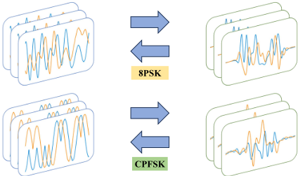
Communication modulation signals contain a wealth of exploitable spectral information with modulation semantics. The extraction of frequency domain features has long been a focus in the field of signal processing [Katsaggelos et al., 1993]. The different modulation schemes exhibit distinct spectral feature distributions in the frequency domain. Figure 1 shows an example of this phenomenon. The spectral energy of the 8PSK modulation scheme is primarily concentrated in the high-frequency region, while the spectral energy of CPFSK is mainly distributed in the mid to lowfrequency range. Inspired by this, we designed a novel selfsupervised training strategy SGSSC that enables the model to learn cross-domain data transformation from time domain to frequency domain. This training strategy allows the model to develop the ability to extract distribution of spectral information with modulation semantics from time-domain signals. To our knowledge, this is a previously unexplored pretext task that is more suitable for communication signal data formats rich in spectral information, compared to generative [He et al., 2022] or contrastive [He et al., 2020] SSL methods. Our approach innovatively uses spectral information to guide the model in learning implicit frequency domain knowledge structures from time-domain data, thereby building a cross-domain knowledge bridge. Additionally, to enhance the model's temporal modeling capability, we employ a masking strategy on the communication signal data within the pretext task. Concurrently, we also recognize that the spectral information inherently carries certain modulation semantics that are closely related to the downstream classification task. Applying a traditional fine-tuning approach on the downstream task may potentially lead to the loss of valuable pre-training knowledge. To address this challenge, we have designed a novel fine-tuning strategy based on attention mechanisms, which enables our model to adaptively integrate different levels of pre-trained features. Our contributions can be summarized as follows:
- We propose a self-supervised training method SGSSC specifically designed for communication signal data, which leverages the spectral information containing modulation semantics in the signals. This approach enables the model to extract deeper semantic features from time-domain data for downstream tasks.
- We introduce a novel fine-tuning strategy based on attention mechanisms for downstream tasks, enabling the adaptive integration of pre-trained features from various levels, thereby preserving valuable knowledge learned during the self-supervised training phase.
- We validated the effectiveness of this self-supervised training framework in downstream communication signal classification tasks. When the proportion of labeled samples is 0.5%, our method achieves an average improvement of 2.3% compared to the best-performing SSL method.
2 RelatedWork
2.1 Signal Classification
Signal classification has long been a pioneering problem in the field of communication. Traditional modulation signal recognition methods rely on manual feature extraction, including spectral features, instantaneous parameter statistical features, and higher-order cumulants [Zhang et al., 2001], as well as likelihood ratio methods for classification tasks [Xu et al., 2011]. However, these methods heavily depend on expert design and signal conditions. With the remarkable achievements of deep learning, a wave of DL-based models has been applied to signal classification. Intuitively, the adopted strategy is to transform signals into a visual format to leverage CV-based models for classification, such as CNN [HuynhThe et al., 2020], RNN [Hong et al., 2017], and Transformer [Hamidi-Rad and Jain, 2021] architectures. The effectiveness of DL-based communication signal classification methods hinges on the availability of a large amount of labeled data. However, in the communication signal field, obtaining labeled data is more challenging compared to the CV field, especially in non-cooperative communication scenarios that require strong expert knowledge. Therefore, correctly handling unlabeled modulation signals is key to successfully completing classification tasks.
2.2 Self-Supervised Learning
SSL primarily leverages pretext tasks to extract supervisory signals from large-scale unlabeled data. In the field of CV, it can be categorized into two types: generativebased methods and contrastive-based methods. The main idea behind generative-based methods is to learn visual features through image generation tasks, such as grayscale image colorization [Zhang et al., 2016], image inpainting [Pathak et al., 2016], and playing image puzzles [Noroozi and Favaro, 2016]. Contrastive-based methods, on the other hand, focus on modeling the relationships between different instances using a simple discriminative structure, examples include SimSiam [Chen and He, 2021], SimCLR [Chen et al., 2020a], and SWAV [Caron et al., 2020a]. Due to the success of contrastive learning methods in the field of CV, some researchers have also introduced them into the field of communication signals [Kong et al., 2023]. However, these methods primarily apply the original algorithmic processes from the CV field, merely altering the model structures or data augmentation methods. They lacked algorithmic innovations tailored to the unique data formats of communication signals or the incorporation of expert knowledge specific to this field.
3 Method
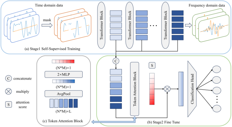
In this section, we will provide an overview of the selfsupervised training framework we have proposed. First, we will introduce the pretext task we have designed specifically for communication signal data. Then, we will elaborate on the masking strategy implemented to further enhance the model's temporal modeling capability for communication signals. Finally, we will present the attention-based finetuning method developed to integrate pre-trained features for downstream tasks. Figure 2 illustrates the complete pipeline of the SGSSC method.
3.1 Pretext Task
The Discrete Fourier Transform (DFT) can be used to analyze the frequency characteristics of signals [Fonseca Guerra et al., 1998], such as identifying the main frequency components in a signal. This is widely applied in fields like audio signal processing and communication system analysis. We leverage the frequency components obtained through the DFT of the time-domain signal x to model Xgt = [X [0] ,X [1] , . . . ,X [L-1]]. Specifically, the p-th component X [p] of the DFT of x is given by the following equation:
where x [k] is the k-th signal value of time-domain signal x. Due to the properties of the DFT, the resulting frequencydomain representation Xgt is a complex vector with the same dimensions as the input time-domain signal x.
Different modulation schemes exhibit distinctly different characteristics in the frequency domain, while signals employing the same modulation schemes tend to have remarkably similar spectral information. We believe that the correlation between modulation schemes and spectral information serves as a powerful prior knowledge, enabling models to better comprehend the inherent modulation semantics of communication signals. Therefore, we designed a simple yet ingenious pretext task. We use the time-domain signal as the input to the model, while the spectrum obtained through the DFT serves as the ground truth to guide the model's training:
where ˜X is the output spectrum predicted by the model. We use Mean Squared Error loss to optimize the model for iterative updates.
By designing a pretext task that encourages the model to learn cross-domain transformations, we enable the model to uncover the intrinsic relationships between the temporal structure of the input signal and the spectral information imbued with modulation semantics. This allows the model to associate its feature representations with the underlying modulation characteristics of the signal. Consequently, in downstream tasks, this holistic understanding empowers the model to extract more fundamental and higher-level features from the time-domain signals, thereby reducing the model's reliance on large amounts of labeled data.
3.2 Masking
In the field of signal classification, enabling models to understand temporal relationships has long been a focus of research. Some scholars have approached this by modifying model architectures, incorporating LSTM [Emam et al., 2020] or Transformer [Cai et al., 2022] modules into models. While this approach equips models with the ability to model the temporal properties of signals, it often lacks a robust loss function to constrain the modeling process. In the fields of CV/NLP, masked autoencoders have proven to be an effective SSL method [Doersch et al., 2015]. This strategy of predicting masked portions allows models to better understand the contextual relationships within data. Inspired by this, we have also introduced the strategy of masking. Specifically, we randomly set certain signal values in the time domain to zero at a certain ratio, and then input these masked signals into the model for pretext task training. Through this approach, the model is forced to leverage the surrounding signal values to infer and reconstruct the masked information. This process encourages the model to develop a more profound understanding of the underlying temporal structure and dependencies within the communication signals.
3.3 Fine-Tuning of AttentionMechanisms
After completing self-supervised training, it is generally believed that the shallow layers of the model capture lowlevel features, while the deeper layers learn features that are strongly related to the pretext tasks [Zhou et al., 2018]. In the field of CV, the pretext tasks often have significant differences from the downstream tasks. Therefore, during finetuning for downstream tasks, it is common practice to use the earlier layers of the complete model as feature extractors [Jing and Tian, 2020], discarding the latter layers of the model structure. However, the SGSSC method differs in this regard. The spectrum of a signal itself possesses inherent modulation semantics, which can be leveraged as features in downstream classification tasks. Consequently, the features at the backend of the model obtained through self-supervised training are closely related to the downstream tasks. Discarding these features would hinder the effective utilization of the knowledge acquired during self-supervised training when fine-tuning for downstream tasks. To address this issue, we design an attention-based fine-tuning approach to integrate features from different layers of the model.
The Figure 2c illustrates the detailed structure of the attention module. In principle, the concept of this module can be embedded in any model architecture. In our case, we primarily integrate the module into the transformer architecture. The model structure we use is similar to the Vision Transformer (ViT) [Dosovitskiy et al., 2020], with simple modifications made to accommodate the data format of signals.
The output of the n-th transformer block in the model can be defined as Fn ∈ R(M×L) , where M is the number of tokens and L is the feature length of each token. The model consists of a total of N transformer blocks. During finetuning, we first concatenate the output features from each layer along the token dimension, resulting in a richer feature representation F ∈ R((N∗M)×L) . This feature incorporates information from different layers, encompassing both low-level features of the signals and high-level features related to the pretext tasks. Next, we employ a token-level attention mechanism to process this feature. There are two main reasons for this approach: firstly, the dimensionality of the feature is quite large, and using it directly for fine-tuning on downstream tasks may easily lead to overfitting, necessitating dimensionality reduction; secondly, the use of tokenlevel attention allows us to selectively focus on and integrate features across different layers and tokens, better leveraging the time-frequency understanding developed during the selfsupervised training phase. This enables the model to seamlessly transfer the learned knowledge to the downstream signal classification task, thereby improving performance. Our specific approach is outlined as follows:
where AvgPool is the average pooling layer. MLP is the fully connected layer, and σ is the sigmoid activation function, which maps the features to values between 0 and 1. The variable A is the attention scores we aim to obtain. Finally, as shown in Equation (4), we multiply each token by its corresponding attention score and then aggregate the results, which serves as the feature representation for the downstream task:
where ˜ F is the input feature for the downstream task.
4 Experiment
4.1 Dataset
We adopted the data generation methodology used in the publicly available RML2016.10a dataset [O'shea and West, 2016] to create datasets under three distinct channel conditions: Additive White Gaussian Noise (AWGN) channel, Rayleigh (Ray) channel, and Rician (Ri) channel. The AWGN channel has additive white Gaussian noise, with the amplitude following a Gaussian distribution and a constant power spectral density function. The Rayleigh channel is used to model scenarios where there is no direct link between the transmitter and receiver, and the signal reaches the receiver through reflection or diffraction. The Rician channel is used to model channel fading situations where there is a direct path and multiple reflected paths simultaneously. Each dataset contains 220,000 modulated signals, comprising
| 0.1% of labeled data | ||||||||||
|---|---|---|---|---|---|---|---|---|---|---|
| AWGN | Rayleigh | Rician | A→Ray | A→Ri | Ray→A | Ray→Ri | Ri →A | Ri →Ray | Average | |
| Random Init | 25.5 | 21.1 | 21.6 | 21.1 | 21.6 | 25.5 | 21.6 | 25.5 | 21.1 | 22.7 |
| Supervised | 28.1 | 23.7 | 23.8 | 23.7 | 23.8 | 28.1 | 23.8 | 28.1 | 23.7 | 25.2 |
| DCL | 37.3 | 26.1 | 24.1 | 25.0 | 25.4 | 31.8 | 24.2 | 28.9 | 26.6 | 27.7 |
| NNCLR | 34.6 | 26.1 | 25.9 | 25.7 | 24.7 | 29.4 | 24.8 | 28.6 | 24.1 | 27.1 |
| SimCLR | 35.0 | 26.8 | 26.3 | 24.1 | 24.1 | 28.7 | 23.9 | 29.5 | 24.8 | 27.0 |
| SimSiam | 32.3 | 27.5 | 27.0 | 26.8 | 24.2 | 32.9 | 25.1 | 31.4 | 25.3 | 28.1 |
| SWAV | 32.9 | 24.0 | 24.5 | 26.1 | 25.6 | 34.1 | 25.6 | 30.8 | 27.4 | 27.9 |
| MAE | 30.7 | 25.4 | 25.2 | 24.4 | 25.0 | 30.6 | 23.5 | 30.2 | 26.0 | 26.8 |
| SSL-ECG | 36.7 | 28.2 | 27.8 | 27.2 | 26.0 | 35.2 | 26.7 | 32.8 | 28.0 | 29.0 |
| CPC | 38.2 | 28.9 | 28.4 | 27.9 | 26.3 | 36.6 | 26.3 | 32.0 | 28.7 | 30.4 |
| TS-TCC | 37.8 | 29.6 | 29.1 | 28.3 | 26.6 | 37.8 | 25.7 | 33.4 | 29.2 | 30.8 |
| InfoTS | 39.5 | 30.3 | 30.0 | 28.7 | 26.8 | 39.0 | 26.0 | 34.1 | 30.5 | 31.7 |
| TimesURL | 40.1 | 31.0 | 30.8 | 29.0 | 27.1 | 39.8 | 27.0 | 34.9 | 31.0 | 32.3 |
| SGSSC* | 39.3 | 29.6 | 30.7 | 28.5 | 26.9 | 39.1 | 27.1 | 33.8 | 30.7 | 31.7 |
| SGSSC | 44.4 | 32.4 | 32.7 | 30.9 | 28.6 | 41.5 | 25.9 | 36.8 | 31.4 | 33.8 |
| 0.5% of labeled data | ||||||||||
| Random Init | 34.1 | 28.8 | 28.4 | 28.8 | 28.4 | 34.1 | 28.4 | 34.1 | 28.8 | 30.4 |
| Supervised | 37.0 | 31.7 | 31.0 | 31.7 | 31.0 | 37.0 | 31.0 | 37.0 | 31.7 | 33.2 |
| DCL | 47.2 | 39.3 | 35.0 | 36.7 | 34.7 | 44.7 | 35.8 | 45.7 | 39.0 | 39.8 |
| NNCLR | 46.7 | 38.5 | 35.4 | 35.9 | 33.2 | 43.8 | 36.1 | 44.6 | 39.4 | 39.3 |
| SimCLR | 46.9 | 38.1 | 34.1 | 35.5 | 33.5 | 43.4 | 35.2 | 44.1 | 38.7 | 38.8 |
| SimSiam | 44.8 | 38.9 | 34.5 | 35.1 | 33.8 | 43.1 | 34.6 | 44.9 | 38.4 | 38.7 |
| SWAV | 47.2 | 40.2 | 34.8 | 36.3 | 34.1 | 44.0 | 34.9 | 45.3 | 38.1 | 39.4 |
| MAE | 47.6 | 39.8 | 35.7 | 37.1 | 34.4 | 44.3 | 35.5 | 46.2 | 39.6 | 40.0 |
| SSL-ECG | 47.5 | 40.6 | 36.0 | 37.5 | 35.0 | 45.0 | 36.7 | 46.4 | 39.9 | 40.5 |
| CPC | 47.7 | 41.0 | 36.3 | 37.9 | 35.3 | 45.3 | 36.4 | 46.9 | 40.5 | 40.8 |
| TS-TCC | 47.7 | 41.4 | 36.6 | 38.3 | 35.6 | 45.6 | 37.0 | 47.3 | 40.2 | 41.1 |
| InfoTS | 47.8 | 41.8 | 37.0 | 38.7 | 35.9 | 45.9 | 37.3 | 47.7 | 40.8 | 41.4 |
| TimesURL | 47.9 | 42.0 | 37.5 | 39.2 | 36.0 | 46.1 | 37.5 | 48.0 | 41.3 | 41.7 |
| SGSSC* | 48.8 | 41.9 | 39.6 | 38.5 | 36.1 | 45.8 | 37.4 | 48.3 | 41.3 | 42.0 |
| SGSSC | 49.5 | 44.0 | 40.4 | 42.0 | 37.9 | 49.0 | 39.5 | 49.8 | 43.8 | 44.0 |
11 modulation schemes, with 20,000 signals per modulation class. The signals are generated at 20 different signal-to-noise ratios (SNR), ranging from -20 dB to 18 dB with a step size of 2 dB. Each class and SNR combination has 1,000 signals.
We further evaluated the effectiveness of our method using six time series datasets: Human Activity Recognition (HAR) [Anguita et al., 2013], Epilepsy Seizure Prediction (ESP) [Andrzejak et al., 2001], and several datasets from the UCR Repository [Dau et al., 2019], including Wafer, PhalangesOutlinesCorrect (POC), ProximalPhalanxOutlineCorrect (PPOC), and StarLightCurves (SLC).
For all datasets, we performed a split, with 60% used for self-supervised training, 20% for validation, and 20% for testing. During fine-tuning on downstream tasks, we randomly sampled the corresponding proportion of data from the selfsupervised training set and utilized their labels.
4.2 Implementation Details
To validate the effectiveness of our method, we followed a standard linear evaluation scheme [Chen et al., 2020b]. In this scheme, a linear classifier (a single fully connected layer) is trained on a frozen self-supervised pre-trained model. In the self-supervised training experiment, we used a mask ratio of 0.7, the Adam optimizer with a learning rate of 0.0001, a batch size of 64, and trained for a total of 500 epochs. For the fine-tuning experiments on downstream tasks, we employed the Adam optimizer, setting the learning rate for the classifier to 0.06 and a batch size of 64. Our model architecture is similar to ViT, with a patch size of 1×16, 8 layers, a hidden size of 128, an MLP size of 1024, and 8 attention heads. All experiments were conducted on a GeForce RTX 3090, and the reported results represent the average performance over five independent runs.
4.3 Overall Performance
To validate the effectiveness of the proposed self-supervised pre-training method SGSSC, we fine-tuned the model on downstream classification tasks using 0.1% and 0.5% of the labeled data, with accuracy as the evaluation metric. The results are shown in Table 1. The experimental datasets encompass various scenarios, including single-channel and cross-channel settings. For instance, "AWGN" indicates both self-supervised training and downstream task fine-tuning are performed on the AWGN dataset, whereas "A → Ray" denotes that self-supervised training is conducted on the AWGN dataset and the downstream classification task is fine-tuned on the Rayleigh dataset. This setup allows us to assess the method's performance on in-distribution tasks as well as its generalization capability in cross-distribution transfer tasks.
To compare performance, we selected 13 comparative methods, categorized into three groups: the baselines include Random Init and Supervised, where Random Init represents training a linear classifier on a frozen and randomly initialized encoder, and Supervised refers to fine-tuning the entire model. DCL [Chuang et al., 2020], NNCLR [Dwibedi et al., 2021], SimCLR [Chen et al., 2020a], SimSiam [Chen and He, 2021], SWAV [Caron et al., 2020b], and MAE [He et al., 2022] are current mainstream self-supervised learning methods in the computer vision domain. SSL-ECG [Sarkar and Etemad, 2020], CPC [Oord et al., 2018], TS-TCC [Eldele et al., 2023], InfoTS [Luo et al., 2023], and TimesURL [Liu and Chen, 2024] are self-supervised learning methods specifically designed for time series data. Additionally, to ensure fairness, we designed a control version SGSSC* that does not employ our proposed attention-based fine-tuning strategy, to validate the pure effectiveness of the feature representations. As shown in Table 1, the proposed SGSSC and SGSSC* methods

| 1% of labeled data | |||||||
|---|---|---|---|---|---|---|---|
| HAR | ESP | Wafer | POC | PPOC | SLC | Average | |
| Random Init | 39.8 | 70.3 | 90.6 | 61.4 | 64.3 | 78.8 | 67.5 |
| Supervised | 44.9 | 76.1 | 91.9 | 62.0 | 68.4 | 80.6 | 70.7 |
| DCL | 58.3 | 86.0 | 93.0 | 61.9 | 68.6 | 80.6 | 74.7 |
| NNCLR | 55.3 | 85.7 | 92.1 | 61.7 | 67.1 | 80.9 | 73.8 |
| SimCLR | 65.8 | 88.3 | 93.8 | 61.5 | 67.6 | 83.6 | 76.8 |
| SimSiam | 61.2 | 84.5 | 92.6 | 62.2 | 67.4 | 80.4 | 74.7 |
| SWAV | 74.9 | 83.2 | 92.4 | 62.5 | 67.8 | 80.1 | 76.8 |
| MAE | 66.8 | 87.3 | 92.8 | 62.8 | 68.2 | 82.3 | 76.7 |
| SSL-ECG | 60.0 | 89.3 | 93.4 | 62.5 | 69.8 | 78.3 | 75.6 |
| CPC | 65.4 | 88.9 | 93.5 | 64.8 | 63.3 | 80.8 | 76.1 |
| TS-TCC | 70.5 | 91.2 | 93.2 | 63.8 | 63.4 | 86.0 | 78.0 |
| InfoTS | 55.9 | 88.4 | 93.3 | 63.0 | 69.3 | 81.2 | 75.2 |
| TimesURL | 64.5 | 89.9 | 93.7 | 63.2 | 68.9 | 81.9 | 77.0 |
| SGSSC* | 70.1 | 89.1 | 93.9 | 63.2 | 69.7 | 81.7 | 77.9 |
| SGSSC | 76.1 | 91.4 | 95.4 | 63.6 | 71.5 | 84.4 | 80.4 |
| 5% of labeled data | |||||||
| Random Init | 49.6 | 75.5 | 91.2 | 61.6 | 64.1 | 74.2 | 69.4 |
| Supervised | 52.8 | 83.4 | 94.6 | 61.4 | 69.1 | 81.8 | 73.9 |
| DCL | 63.2 | 90.4 | 93.9 | 61.3 | 71.5 | 83.9 | 77.4 |
| NNCLR | 60.5 | 85.6 | 93.4 | 61.7 | 72.3 | 82.3 | 76.0 |
| SimCLR | 75.8 | 91.3 | 94.8 | 62.7 | 68.0 | 84.2 | 79.5 |
| SimSiam | 65.3 | 84.1 | 94.2 | 61.1 | 73.1 | 83.0 | 76.8 |
| SWAV | 68.4 | 87.3 | 94.7 | 61.5 | 70.2 | 85.1 | 77.9 |
| MAE | 70.6 | 89.0 | 95.5 | 61.6 | 70.9 | 86.8 | 79.1 |
| SSL-ECG | 63.7 | 92.8 | 94.9 | 62.9 | 68.8 | 82.6 | 77.6 |
| CPC | 75.4 | 92.8 | 92.5 | 66.9 | 71.5 | 89.1 | 81.4 |
| TS-TCC | 77.6 | 93.1 | 93.2 | 63.8 | 72.1 | 89.6 | 81.6 |
| InfoTS | 73.1 | 92.2 | 95.8 | 61.9 | 73.8 | 87.2 | 80.7 |
| TimesURL | 76.8 | 94.8 | 96.9 | 62.0 | 74.4 | 88.5 | 78.9 |
| SGSSC* | 79.2 | 93.5 | 96.1 | 61.8 | 74.9 | 88.7 | 82.4 |
| 85.3 | |||||||
| SGSSC | 85.1 | 96.6 | 98.8 | 62.6 | 77.3 | 91.7 | |
(a) 0.1% of labeled data
(b) 0.5% of labeled data
achieve superior performance across all experimental scenarios.
Furthermore, to demonstrate the potential of our method on time series data, we conducted experiments on six time series datasets. For these datasets, we fine-tuned the model using 1% and 5% of the labeled data. The experimental results, presented in Table 2, indicate that our method outperforms others on five of these datasets as well as in terms of the average accuracy across all datasets.
4.4 Mask Ratio
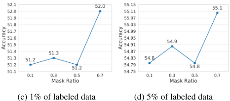
To investigate the impact of different mask ratios in selfsupervised training on downstream task performance, we set mask ratio to 0.1, 0.3, 0.5, and 0.7, and conducted selfsupervised training on the AWGN dataset. Figure 3 shows the frequency-domain reconstruction quality of a BPSK modulation scheme with a SNR of 18 dB under different mask ratios. As observed, increasing the mask ratio leads to degradation in reconstruction details. Nevertheless, the overall frequency distribution characteristics are still well preserved.
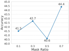
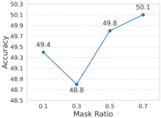
Figure 4 presents the experimental results of models trained with different mask ratio on downstream tasks. It is evident that when the mask ratio is 0.7, the model demonstrates excellent feature extraction capabilities. This is because the signal data exhibits strong temporal continuity with minimal fluctuations. At lower mask ratios, the model tends to learn shortcuts in temporal modeling, while only at higher mask ratios is the model compelled to discover more robust features within the signal, thus facilitating the effective transfer of knowledge to the downstream tasks.

| DCL | NNCLR | SimCLR | SimSiam | SWAV | MAE | SSL-ECG | CPC | TS-TCC | InfoTS | TimesURL | SGSSC | |
|---|---|---|---|---|---|---|---|---|---|---|---|---|
| MFLOPs | 1.147 | 1.547 | 1.147 | 1.430 | 1.214 | 1.586 | 1.595 | 1.632 | 1.437 | 1.865 | 1.743 | 1.606 |
| Params/M | 1.117 | 1.513 | 1.117 | 1.397 | 1.183 | 1.174 | 1.478 | 1.617 | 1.398 | 1.871 | 1.710 | 1.185 |
4.5 Visualization and Computational Complexity
To more intuitively demonstrate the allocation of feature weights by our proposed attention-based fine-tuning strategy, we visualized the attention weights across different layers of the model, with the results presented in Figure 5. In the visualization, the horizontal axis represents the attention weights of different tokens in the model arranged in the order of forward propagation layers, while the vertical axis corresponds to datasets from three channel environments. From the figure, it can be observed that tokens from deeper layers exhibit significantly higher attention values, whereas those from shallower layers have relatively lower attention values. This aligns with the objective of our proposed fine-tuning strategy, indicating that the token-level attention mechanism can selectively focus on high-level features that are closely related between the pretext task and downstream task, while retaining low-level features from shallow layers to provide foundational information.
Meanwhile, we also calculated the computational cost in FLOPs and the number of parameters for our method and the comparative methods discussed in this paper, with the results shown in Table 3. As seen in the table, our method has computational and parameter counts similar to some of the current mainstream approaches. This is because the pretext task we designed are very simple, and the attention-based fine-tuning strategy only adds a few small linear layers, resulting in minimal overhead.
4.6 Ablation Experiment
We conducted an ablation study on the attention mechanism and masking strategy using three datasets, with an experimental setting of 0.1% labeled data for downstream tasks. Table
| Dataset | Supervised | w/attention | w/mask | w/atttenion+mask |
|---|---|---|---|---|
| AWGN | 28.1 | 35.4(+7.3) | 39.3(+11.2) | 44.4(+16.3) |
| Rayleigh | 23.7 | 28.2(+4.5) | 29.6(+5.9) | 32.4(+8.7) |
| Rician | 23.8 | 27.0(+3.2) | 30.7(+6.9) | 32.7(+8.9) |
4 presents the ablation results. The table shows that incorporating all components improves performance compared to the baseline. On the AWGN dataset, adding only the attention mechanism without masking the time-domain data leads to a 7.3% performance increase. Using a masking ratio of 0.7 on the time-domain data without the attention mechanism results in a 11.2% performance boost. When both modules are employed simultaneously, the model's performance increases by 16.3%. These findings indicate that both modules contribute significantly to the model's performance, facilitating efficient knowledge transfer to downstream tasks. The attention mechanism helps the model focus on features highly relevant to the downstream task, while the masking strategy encourages the model to learn more robust temporal modeling from partially masked time-domain signals.
5 Conclusion
Acquiring labels for communication signal data is often a challenging task. To address this issue, this paper explores a self-supervised learning method called Spectral-Guided SelfSupervised Signal Classification, which is particularly suited for time series data with rich spectral information. By leveraging spectral information, this method facilitates the model's learning of more prior knowledge with modulation semantics. To validate its effectiveness, we conducted experiments using both signal and time series datasets, demonstrating that this training approach aids the model in acquiring richer feature representations and achieving superior performance in downstream tasks. We hope that this self-supervised learning method will advance research across various time series domains.
@inproceedings{ijcai2025p752,
  title     = {Predicting Spectral Information for Self-Supervised Signal Classification},
  author    = {Xu, Yi and Wang, Shuang and Xing, Hantong and Wang, Chenxu and Quan, Dou and Yang, Rui and Zhao, Dong and Mei, Luyang},
  booktitle = {Proceedings of the Thirty-Fourth International Joint Conference on
               Artificial Intelligence, {IJCAI-25}},
  publisher = {International Joint Conferences on Artificial Intelligence Organization},
  editor    = {James Kwok},
  pages     = {6758--6766},
  year      = {2025},
  month     = {8},
  note      = {Main Track},
  doi       = {10.24963/ijcai.2025/752},
  url       = {https://doi.org/10.24963/ijcai.2025/752},
}
TY - CPAPER TI - Predicting Spectral Information for Self-Supervised Signal Classification AU - Xu, Yi AU - Wang, Shuang AU - Xing, Hantong AU - Wang, Chenxu AU - Quan, Dou AU - Yang, Rui AU - Zhao, Dong AU - Mei, Luyang T2 - Proceedings of the Thirty-Fourth International Joint Conference on Artificial Intelligence, IJCAI-25 PB - International Joint Conferences on Artificial Intelligence Organization PY - 2025 SP - 6758 EP - 6766 DO - 10.24963/ijcai.2025/752 UR - https://doi.org/10.24963/ijcai.2025/752 ER -Copied
Machine-readable versions of this paper, for tools and AI agents:





