
Run Like a Neural Network, Explain Like k-Nearest Neighbor
Proceedings of the Thirty-Fourth International Joint Conference on Artificial Intelligence. Main Track. Pages 6857-6865.
https://doi.org/10.24963/ijcai.2025/763
Keywords
- Knowledge Representation and Reasoning: KRR: Case-based reasoning
- Machine Learning: ML: Explainable/Interpretable machine learning
- Machine Learning: ML: Feature extraction, selection and dimensionality reduction
- Machine Learning: ML: Neuro-symbolic methods/Abductive Learning
Abstract
Deep neural networks have achieved remarkable performance across a variety of applications. However, their decision-making processes are opaque. In contrast, k-nearest neighbor (k-NN) provides interpretable predictions by relying on similar cases, but it lacks important capabilities of neural networks.
The neural network k-nearest neighbor (NN-kNN) model is designed to bridge this gap, combining the benefits of neural networks with the instance-based interpretability of k-NN. However, the initial formulation of NN-kNN had limitations including scalability issues, reliance on surface-level features, and an excessive number of parameters. This paper improves NN-kNN by enhancing its scalability, parameter efficiency, ease of integration with feature extractors, and training simplicity.
An evaluation of the revised architecture for image and language classification tasks illustrates its promise as a flexible and interpretable method.
- [Adadi and Berrada, 2018] Amina Adadi and Mohammed Berrada. Peeking inside the black-box: A survey on explainable artificial intelligence (xai). IEEE Access, 6:52138-52160, 2018.
- [An et al., 2018] Shuai An, Jun Wang, and Jinmao Wei. Local-nearest-neighbors-based feature weighting for gene selection. IEEE/ACM Transactions on Computational Bi- ology and Bioinformatics, 15(5):1538-1548, 2018.
- [Bellet et al., 2015] A. Bellet, A. Habrard, and M. Sebban. Metric Learning. Synthesis Lectures on Artificial Intel- ligence and Machine Learning. Morgan & Claypool Pub- lishers, 2015.
- [Bicego and Loog, 2016] M. Bicego and M. Loog. Weighted k-nearest neighbor revisited. In Twenty-Third Interna- tional Conference on Pattern Recognition (ICPR), pages 1642-1647. IEEE, 2016.
- [Cover and Hart, 1967] T. Cover and P. Hart. Nearest neigh- bor pattern classification. IEEE Transactions on Informa- tion Theory, 13:21-27, 1967.
- [Dua and Graff, 2017] D. Dua and C. Graff. UCI machine learning repository, 2017.
- [Goldberger et al., 2004] Jacob Goldberger, Geoffrey E Hin- ton, Sam Roweis, and Russ R Salakhutdinov. Neighbour- hood components analysis. In Advances in Neural Infor- mation Processing Systems, volume 17. MIT Press, 2004.
- [Guidotti et al., 2018] Riccardo Guidotti, Anna Monreale, Salvatore Ruggieri, Franco Turini, Fosca Giannotti, and Dino Pedreschi. A survey of methods for explaining black box models. ACM Comput. Surv., 51(5), August 2018.
- [He et al., 2016] Kaiming He, Xiangyu Zhang, Shaoqing Ren, and Jian Sun. Deep residual learning for image recog- nition. In 2016 IEEE Conference on Computer Vision and Pattern Recognition (CVPR), pages 770-778, 2016.
- [Jalali and Leake, 2018] V. Jalali and D. Leake. Harnessing hundreds of millions of cases: Case-based prediction at industrial scale. In Case-Based Reasoning Research and Development, ICCBR 2018, Berlin, 2018. Springer.
- [Johnson et al., 2019] Jeff Johnson, Matthijs Douze, and Hervé Jégou. Billion-scale similarity search with GPUs. IEEE Transactions on Big Data, 7(3):535-547, 2019.
- [Keane and Kenny, 2019] Mark T. Keane and Eoin M. Kenny. How case-based reasoning explains neural net- works: A theoretical analysis of XAI using post-hoc explanation-by-example from a survey of ANN-CBR twin-systems. In Case-Based Reasoning Research and De- velopment, pages 155-171, Cham, 2019. Springer.
- [Krizhevsky, 2009] Alex Krizhevsky. Learning multiple lay- ers of features from tiny images. Technical report, Univer- sity of Toronto, 2009.
- [Kulis, 2013] Brian Kulis. Metric learning: A survey. Found. Trends Mach. Learn., 5:287-364, 2013.
- [Le and Mikolov, 2014] Quoc Le and Tomas Mikolov. Dis- tributed representations of sentences and documents. In Proceedings of the 31st International Conference on Ma- chine Learning, volume 32, pages 1188-1196, Bejing, China, 22-24 Jun 2014. PMLR.
- [Leake and Ye, 2021] David Leake and Xiaomeng Ye. Har- monizing case retrieval and adaptation with alternating op- timization. In Case-Based Reasoning Research and Devel- opment, ICCBR 2019, pages 125-139. Springer, 2021.
- [Li et al., 2018] Oscar Li, Hao Liu, Chaofan Chen, and Cynthia Rudin. Deep learning for case-based reasoning through prototypes: A neural network that explains its pre- dictions. In Proceedings of the Thirty-Second AAAI Con- ference on Artificial Intelligence, pages 3530-3537. AAAI Press, 2018.
- [Netzer et al., 2011] Yuval Netzer, Tao Wang, Adam Coates, Alessandro Bissacco, Bo Wu, and Andrew Y. Ng. Reading digits in natural images with unsupervised feature learn- ing. In NIPS Workshop on Deep Learning and Unsuper- vised Feature Learning 2011, 2011.
- [Park et al., 2004] Jae Park, Kwang Hyuk Im, Chung-Kwan Shin, and Sang Park. Mbnr: Case-based reasoning with local feature weighting by neural network. Applied Intel- ligence, 21, 11 2004.
- [Ricci and Avesani, 1995] F. Ricci and P. Avesani. Learning a local similarity metric for case-based reasoning. In Pro- ceedings of the First International Conference on Case- Based Reasoning, pages 301-312, Berlin, 1995. Springer Verlag.
- [Rudin et al., 2022] Cynthia Rudin, Chaofan Chen, Zhi Chen, Haiyang Huang, Lesia Semenova, and Chudi Zhong. Interpretable machine learning: Fundamental prin- ciples and 10 grand challenges. Statistic Surveys, 16:1-85, 2022.
- [Rudin, 2019] Cynthia Rudin. Stop explaining black box machine learning models for high stakes decisions and use interpretable models instead. Nature Machine Intelligence, 1:206-215, 05 2019.
- [Weinberger and Saul, 2009] Kilian Q. Weinberger and Lawrence K. Saul. Distance metric learning for large margin nearest neighbor classification. J. Mach. Learn. Res., 10:207-244, jun 2009.
- [Wettschereck et al., 1997] D. Wettschereck, D. Aha, and T. Mohri. A review and empirical evaluation of feature- weighting methods for a class of lazy learning algorithms. Artificial Intelligence Review, 11(1-5):273-314, February 1997.
- [Ye et al., 2024] Xiaomeng Ye, David Leake, Yu Wang, Zi- wei Zhao, and David Crandall. Towards network imple- mentation of CBR: Case study of a neural network K- NN algorithm. In Case-Based Reasoning Research and Development, ICCBR 2024, pages 354-370, Cham, 2024. Springer.
References were extracted automatically from the PDF and may contain errors.
Full text extracted automatically from the PDF; figures, tables and equations may differ. The PDF is the version of record.
1 Introduction
The importance of explaining AI system behavior is widely acknowledged. The dominance of neural network models has prompted numerous efforts to develop explanation components that provide post-hoc explanations of neural systems [Guidotti et al., 2018; Adadi and Berrada, 2018]. However, Rudin et al. [2022] advocate a different path: developing inherently interpretable models rather than relying on post-hoc explanations for black-box models. They argue that post-hoc explanations often fail to accurately reflect the reasoning process of black-box models, potentially misleading users. In contrast, inherently interpretable models enhance trust and can expose potential flaws in the data, which is particularly advantageous in high-stakes applications.
The k-nearest neighbor (k-NN) algorithm is a classic interpretable algorithm. It predicts the label of a query by analyzing the k most similar instances from previously observed data and combining their results, generally by straightforward methods such as averaging or majority vote [Cover and Hart, 1967]. The k-NN decision-making process, directly influenced by neighboring data points, enables intuitive, instance-based explanations. Despite its simplicity, k- NN has demonstrated competitive performance across diverse datasets, often achieving accuracy comparable to more complex machine learning models [Rudin, 2019]. However, its effectiveness depends heavily on factors such as feature selection, distance measures, instance weighting, and feature weighting. This poses challenges when fine-tuning the model for more complex datasets [Kulis, 2013; Park et al., 2004; Weinberger and Saul, 2009; Bellet et al., 2015]. More recent variations of k-NN, such as Large Margin Nearest Neighbor (LMNN) [Weinberger and Saul, 2009] and Neighborhood Components Analysis (NCA) [Goldberger et al., 2004], partially address these challenges by learning transformations of the feature space to improve classification accuracy.
However, k-NN struggles with high-dimensional or largescale data due to the cost of exhaustive comparisons, difficulty in feature selection, and the curse of dimensionality. Various efforts tackle these challenges [Jalali and Leake, 2018; Johnson et al., 2019]. In contrast, neural networks excel at capturing abstract representations, hidden patterns, and the relative importance of features in high-dimensional spaces. They also leverage tensor computations and parallel computing to handle large datasets. The contrasting strengths and weaknesses of k-NN and network models make it appealing to develop hybrids harnessing the strengths and alleviating the weaknesses of each. For example, Li et al. [2018] propose a model in which a prototype layer stores embeddings of learned prototypes and uses them in classification. Because the network relies on the prototype layer for classification, its decision can be interpreted in terms of activated prototypes.
Inspired by Li et al. [2018], Ye et al. [2024] introduced neural network based k-nearest neighbor (NN-kNN), a hybrid model aiming to provide both the interpretability of k-NN and the learning capabilities of neural networks. The NN-kNN architecture reimagines the k-NN process within a neural network framework, integrating feature extraction, similarity assessment, and prediction into a cohesive, end-to-end trainable model. This design enables NN-kNN to simultaneously learn feature importance [Wettschereck et al., 1997], case weights [Bicego and Loog, 2016], and distance metrics, enhancing its adaptability and performance.
The initial NN-kNN provided multiple benefits, but it also had limitations: (1) As datasets grow in size and complexity-as for natural images or text embeddings-the computational cost of comparing a query to every stored case becomes prohibitive,
(2) Its reliance on raw features limits its ability to capture hidden patterns effectively, and (3) Its feature weighting scheme either assigned identical weightings to all cases, or assigned unique weightings to each case. This method could underfit by neglecting local patterns or overfit by assigning weights too specifically to individual instances.
This paper presents work on extending NN-kNN to address these limitations. Our key contributions include:
- Scalability by Case Sampling. We introduce a sampling mechanism that selects a subset of cases to use during training and inference, significantly reducing computational cost.
- Feature Extraction for High-Dimensional Data. We integrate a feature extraction layer in NN-kNN, which can be either pretrained or jointly trained end-to-end with NN-kNN. This enables NN-kNN to effectively process high-dimensional data, expanding its applicability to domains like image classification and NLP.
- Global-local ("Glocal") Feature Weighting Scheme. We present a feature weighting mechanism that combines global feature weights with case-specific coefficients to compute adaptive weights for each case. This reduces the number of parameters while maintaining flexibility.
- Activation Function for Differentiable k-NN. We created a custom differentiable activation function for kNN. Cases within a chosen proximity activate, while other cases have near-zero activations.
- Evaluation on Image and Language Benchmarks. To validate the effectiveness of our extended NN-kNN, we conduct experiments on natural image classification and language classification. NN-kNN both predicts and explains its predictions using the top activated cases.
Our results support that the extended NN-kNN retains the intuitive, case-driven explanations of traditional k-NN while addressing critical previous limitations. By bridging the gap between classical k-NN and neural networks and integrating with state-of-the-art neural feature extractors, NN-kNN provides functionality for interpretable and scalable systems.
2 RelatedWork: Metric Learning and the Original NN-kNN Model
A simple k-NN approach assumes that all features contribute equally to the distance calculation and that all cases are equally important in the domain space. Wettschereck et al. [1997] present a more general distance calculation, and extensive research on distance metric learning has produced numerous k-NN variants [Bellet et al., 2015; Kulis, 2013; Park et al., 2004; Bicego and Loog, 2016]. Among these, Neighborhood Components Analysis (NCA) [Goldberger et al., 2004] and Large Margin Nearest Neighbor (LMNN) [Weinberger and Saul, 2009] are particularly notable for their ability to learn linear transformations of the feature space, enhancing classification accuracy.
The neural network based k-nearest neighbor (NN-kNN) model [Ye et al., 2024] reimagines the k-NN process within a neural network architecture. Its architecture computes feature distances, case activations, and class activations in a sequential manner. This design enables NN-kNN to learn feature importance, case weights, and distance metrics directly from data in an end-to-end training process, while remaining interpretable as the intuitive, instance-based reasoning of traditional k-NN. The model has shown competitive performance with neural networks in basic classification and regression tasks. However, the original NN-kNN model faced several limitations, for scalability to large datasets, handling highdimensional data, and restricted feature-weighting options. This paper presents an extended model addressing these issues. To differentiate the old and new models, we will refer to the original as NN-kNNO.
3 Design of the Extended NN-kNN
We extend NN-kNNO for large-scale and high-dimensional datasets. Each case c is associated with a default activation strength biasc (indicating the range of queries that activate the case), a case weight (indicating the extent to which case activates a class) and a one-hot encoded class label. Figure 1 illustrates the overall workflow of NN-kNN, as explained below. Only in step 3 is the process identical to NN-kNNO.
- Sampling Cases for Comparison: A query q is compared with a subset of cases from each class.
- Extracting Features: The feature extraction layer maps input x (a query or a case) to a d-dimensional vector, f(x) =< x1, x2, ..., xd >. For example, ResNet can be used for image data [He et al., 2016], and doc2vec for text data [Le and Mikolov, 2014].
- Calculating Feature Distances: The feature distance layer δ measures distance between each corresponding feature j of the query q and the case c as δj(qj, cj) (abbreviated as δj). In this work, we use Euclidean distance.
- Summing Weighted Feature Distances: Each feature distance δj is scaled based on its importance cwj (see Section 3.1). The weighted distances are summed to compute the overall distance between q and c.
- Activating the Case c: Case c's activation is calculated based on a function of the difference between biasc and the distance from q (see Section 3.2).
- Activating the Class: The case activation is multiplied by the case weight and its one-hot encoded label to contribute to the class activation. The sum of class activations is calculated for all cases, and the class with the maximum activation is chosen as the prediction.
3.1 Global-Local FeatureWeighting
In NN-kNNO, all cases either share a single global feature weighting or each has an individual feature weighting. The later approach tends to perform better because the model can learn to adjust to local landscapes in the task domain [Ricci and Avesani, 1995; An et al., 2018], but at the cost of many parameters to learn.
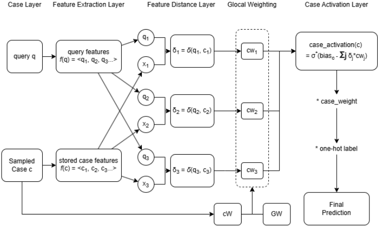
We introduce a global-local (glocal) feature weighting mechanism that bridges the gap between global and individualized weightings. The glocal approach enables tuning the amount of locality in weightings; from global to completely local. This flexibility enables balancing trade-offs in accuracy, storage, and weight learning costs.
We consider cases characterized by vectors of scalar features within a feature space of dimension d. This scheme uses a shared set of w global feature weights GW = {GW1,GW2, ...,GWw} where each set GWi = {wi1,wi2, ...,wid} is a vector of length d. The weight wij represents the importance of feature j according to the global weighting GWi. Each case c is associated with its own set of learnable coefficients cW = {cW1, cW2, ..., cWw}. Intuitively, cWi quantifies how strongly case c is influenced by the global weighting GWi.
The feature weights cw (different from cW) for a specific case c are calculated as the dot product of the coefficients cW and the global feature weights GW.
Testbed System Implementation Details
In the testbed system used for our experiments,
This equation computes the feature weights cw of shape 1 × d by the dot product of the case-specific coefficients cW (1 × w) and the global weights GW (w × d). A leakyReLU is applied here to ensure that all feature weightings in cw stay positive or close to 0. This design maintains the k-NN property that feature differences monotonically increase case distances. If there is a single global feature weight (w = 1), feature weights are initially set to w1j = 1 for every j, ensuring equal importance prior to training. If there are more global feature weights (w ̸= 1), the weights wij are randomly initialized within [0, 1].
When d ≫ w, this design significantly reduces the parameter count for each case from d to w, enhancing computational efficiency while preserving the ability to capture local characteristics of the case space.
3.2 Case Activation Function
Traditionally, k-NN uses the parameter k to specify the number of neighbors to consider. NN-kNN uses a case activation function to distinguish between relevant and irrelevant cases. Let each case's biasc be initialized as B, the initial range of activation. NN-kNN uses a special scaled sigmoid function as the case activation function,
where σ(a) is the standard sigmoid function,
The scaled sigmoid function σ∗ (a) maps the raw case activation values from [-∞. . . biasc] to the range [0, 1]. Cases identical to the query achieve the highest activation because Σj(δjcwj) = 0, resulting in σ∗ (biasc) ≃ σ∗ (B) ≃ 1. Conversely, cases with distances exceeding biasc yield low activations, as a < 0 and σ∗ (a) < σ(-4) ≃ 0. Without scaling, the raw activation may over-saturate a sigmoid function with its gradient plateaued to 0, making the training process difficult.
This activation function offers significant advantages over the traditional parameter k for the following reasons:
- Consistency: B provides more consistent retrieval than k. Simply selecting the top k nearest neighbors disregards the relative distances of these neighbors to the query (distance-weighting can be applied but does not truly address this). For example, if the query is far from training cases, then selecting its top k nearest neighbors may retrieve cases far away from the query, while selecting cases within range B will only retrieve cases nearby.
- Case-Specific Customization: biasc is individually tailored to each case c. A case with a high biasc indicates a larger radius of activation, or the ability to activate for a wider range of queries.
- Trainability: Unlike a fixed parameter k, biasc can be trained to optimize the performance of the model.
Testbed System Implementation Details
In our experiments, we initialize biasc = B as the average unweighted distance of the k-th nearest neighbor in all cases. Under this setting, on average, cases farther from the query's k-th nearest neighbor will not be activated, as their case distances will be larger than biasc. Conversely, cases within the k-th nearest neighbor will be activated.
4 Experimental Evaluation
Computational experiments are carried out to test two main hypotheses:
- NN-kNN using glocal feature weighting retains accuracy comparable to that of NN-kNNO using either global or individual feature weighting.
- NN-kNNusing sampling and feature extraction achieves comparable accuracy to neural counterparts on larger datasets, while providing instance-based explanations.
4.1 Settings and Implementation
To evaluate the impact of varying parameters, we test various k and w until best performance is found. The default case activation B is determined by the average distance to the k-th nearest neighbor across all cases, and w represents the number of global feature weights. All experimental results are summarized but only experimental results providing interesting insights are shown due to space. 1
For datasets with predefined train-test splits, we use the provided partitions. For datasets without such splits, we create a 90-10 train-test split. All models, including NN-kNN and the baseline models, are trained until testing accuracy stabilizes, defined as no improvement for 40 epochs (referred to as the training patience). This evaluation approach is applied consistently across all models for fair comparison. A more robust approach would train until validation accuracy plateaus within the training patience and then measure testing accuracy, but this is not feasible for smaller datasets as splitting the training set further into a validation set could significantly reduce the size of both subsets, potentially destabilizing training and leading to unreliable results.
1 All code can be found on https://github.com/Heuzi/NN-kNN
| features | samples | classes | |
|---|---|---|---|
| Iris | 4 | 150 | 3 |
| Zebra (a) | 2 | 110 | 2 |
| Zebra (b) | 2 | 220 | 2 |
| Wine | 13 | 178 | 3 |
| Breast Cancer | 30 | 569 | 2 |
| Balance | 4 | 625 | 3 |
| Digits | 64 | 1797 | 10 |
For smaller datasets, we use 10-fold cross-validation; for larger datasets, we conduct 10 iterations on the given traintest split. The mean and standard deviation of accuracy are reported. For NN-kNN, if all training cases cannot fit into memory, we sample a subset of cases evenly across all classes.
4.2 Parameter Settings
We trained baseline models (e.g., convolutional image classifiers), with a learning rate of 1e-4 . For NN-kNN without a feature extractor on small datasets (Section 5.1), we set the learning rate to 1e-2 , as it provided the fastest convergence and helped avoid local minima. For NN-kNN on larger datasets, we used varying learning rates tailored to different components of the model: 1e-4 for the feature extractor, 1e-3 for the glocal weighting parameters, and 1e-4 for case-related parameters such as case biasc and case weight. These choices were guided by experimental observations: the glocal weighting parameters benefit from larger steps to converge faster and avoid local minima; the feature extractor requires fine-tuning, similar to traditional neural network classifiers; and the case-related parameters need smaller learning rates to prevent early overfitting, which could overshadow the training of the rest of the model.
5 Experimental Results
5.1 Comparison with NN-kNNO
The first experiments for classification tasks parallel those in the NN-kNNO study [Ye et al., 2024]. All data sets (see Table 1) are from UCI repository [Dua and Graff, 2017] except Zebra (a) and Zebra (b), which are explained later. Table 2 shows the classification accuracies of the models. F1 scores are not shown as the data sets are balanced and F1 shows a consistent pattern with accuracy scores. NN-kNNO allows a few parameter settings such as whether to allow only the top k cases to contribute to class activation and whether all cases share a single global weighting or each case have its own individual weighting. For comparison, we include the previously reported best results by NN-kNNO and a standard neural network classifier with 4 hidden layers using leakyReLU activation functions.
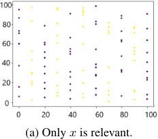
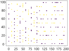
The most notable experimental results concern the Zebra Stripe datasets. They are two synthetic datasets, named Zebra (a) and Zebra (b), where each sample has two attributes x and y and one of two class labels, illustrated in Figure 2. In Zebra (a), only the feature x is relevant; In Zebra (b), x is relevant if x < 100 otherwise y is relevant. The classes are distributed interchangeably along the axis of the relevant feature. These datasets may appear deceptively simple. Standard neural networks, k-NN, NCA, LMNN all fail to capture the essence of the model and have poor accuracies (most < 70%), with the exception that NCA achieved 98.1% for Zebra (a). In tests, NN-kNN manages to learn the ideal feature weights. For example, when using w ≥ 2 on Zebra (b), it learns a feature weight that ignores x and another that ignores y.
| w=1 | w=4 | k | NN-kNNO | NNet | |
|---|---|---|---|---|---|
| Iris | 0.980 (0.031) | 0.973 (0.044) | 5 | 0.966 | 0.987 |
| Zebra (a) | 0.945 (0.164) 0.800 (0.172) | 0.964 (0.073) 0.982 (0.036) | 1 5 | 0.918 | 0.782 |
| Zebra (b) | 0.764 (0.057) 0.718 (0.076) | 0.923 (0.041) 0.932 (0.047) | 1 5 | 0.968 | 0.673 |
| Wine | 0.922 (0.075) 0.838 (0.103) | 0.972 (0.038) 0.843 (0.110) | 1 5 | 0.994 | 0.836 |
| Breast Cancer | 0.986 (0.019) | 0.984 (0.018) | 5 | 0.959 | 0.951 |
| Balance | 0.942 (0.025) | 0.952 (0.032) | 5 | 0.944 | 0.994 |
| Digits | 0.983 (0.008) | 0.986 (0.010) | 5 | 0.988 | 0.983 |
The results suggest the following key findings:
- NN-kNN generally outperforms NN-kNNO, except for Zebra (b) and Wine. This discrepancy arises because NN-kNNO allows individual case weighting, which can be advantageous in scenarios where multiple local landscapes deviate significantly from the global trend.
- Increasing w consistently improves the performance of NN-kNN. Additional global weightings allow the model to adapt to more hidden patterns within the feature space.
- The choice of k has a significant impact on performance. A poorly chosen initial default bias can result in either too many or too few cases being activated, which hinders the model's ability to learn effectively during training.
5.2 Image Classification
To test the effectiveness of NN-kNN with a feature extractor on image tasks, we carried out experiments on CIFAR-10 [Krizhevsky, 2009] and SVHN [Netzer et al., 2011]. CIFAR10 contains natural images of 10 classes such as airplanes, frogs, cats, etc., while SVHN contains images of house number digits from natural street views, also with 10 classes (one for each digit). CIFAR-10 consists of 60,000 images of dimension 3x32x32 (channel x width x height). The dataset has a preset partition of 50,000 training samples and 10,000 testing samples. Similarly, SVHN contains images of the same dimensions as CIFAR-10 and is divided into 73,257 images for training and 26,032 images for testing. The mean and standard deviation of all image pixels are computed across all images and channels in the training dataset. These statistics are used to standardize the pixel values for both the training and testing datasets.
| Method | CIFAR-10 | SVHN |
|---|---|---|
| Conv + NN-kNN 500 | 0.688 (0.006) | 0.867 (0.003) |
| Conv + NN-kNN 2000 | 0.675 (0.003) | 0.841 (0.008) |
| ConvNet | 0.689 | 0.875 |
| kNN | 0.339 | 0.469 |
| Pre-Conv + kNN | 0.647 | 0.869 |
| Pre-Conv + NN-kNN | 0.585 | 0.75 |
Table 3: Accuracies of Different Methods on Image Classification Tasks. "Conv" stands for convolutional layer for feature extractor. "ConvNet" stands for standard convolutional neural network classifier. "Pre-Conv" stands for convolutional layer pretraiend from "ConvNet" and parameters are frozen after training.
For comparison, we used a convolutional neural network (CNN) with the following architecture: two convolutional layers, each followed by ReLU activation and max pooling. The first convolutional layer uses 32 filters with a kernel size of 3 and padding of 1, while the second uses 64 filters with the same configuration. After the convolutional and pooling layers, the feature map is flattened and passed through a fully connected layer with 128 units and ReLU activation, followed by a final output layer with 10 units (one for each class).
We use the layers of the CNN up to the penultimate layer as the feature extractor for both NN-kNN and vanilla k-NN. For NN-kNN, we experimented with the setting w = 1, k = 20 and sampling 500 and 2000 cases for each query. We experimented with two approaches for feature extractors of NNkNN: using a frozen pretrained CNN, or training the CNN alongside NN-kNN from scratch. In contrast, because k-NN cannot jointly train with the feature extractor, we use a frozen pretrained CNN as the feature extractor for k-NN.
Classification Accuracy
The results are presented in Table 3. We observe that NNkNN and ConvNet have comparable accuracy. While using a pretrained feature extractor significantly improves the performance of k-NN, NN-kNN tends to overfit when using pretrained feature extractors. This suggests that training the feature extractor jointly with NN-kNN allows it to be better optimized for instance-based reasoning, enabling NN-kNN to fine-tune feature weights and further enhance accuracy. Notably, "Conv + NN-kNN" performs better than "Pre-Conv + kNN" in CIFAR-10 but equally well in SVHN. We believe that this is because SVHN is an easier data set and the features extracted by pretrained "ConvNet" are sufficient for k-NN to use for instance-based reasoning.
NN-kNN also demonstrates robustness in the presence of misclassification. For instance, in one experiment on CIFAR10, NN-kNN achieves an accuracy of 67.2%. The true class label is among the top 2 activated classes 82.02% of the time and within the top 3 classes 89.96% of the time. This highlights NN-kNN's ability to provide meaningful predictions even when the final classification is incorrect.
Interpretability
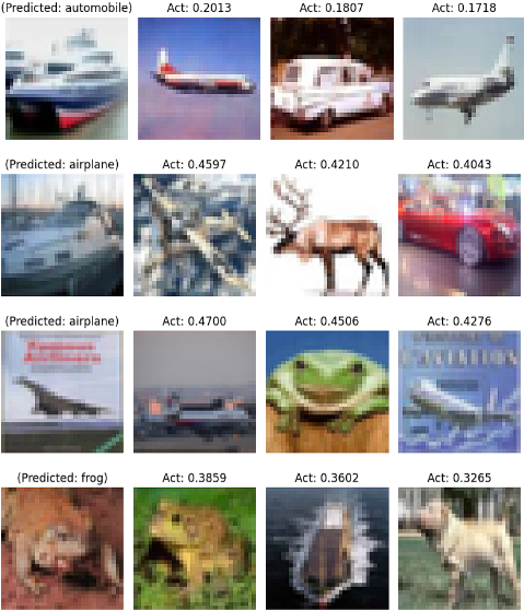
NN-kNN provides interpretable predictions by explaining its decisions based on the activated cases. Unlike post-hoc explanations of neural network decisions by cases [Keane and Kenny, 2019], where similar cases are retrieved after a prediction is made, the activated cases in NN-kNN directly lead to the prediction. Examples of these explanations in CIFAR10 are illustrated in Figure 3. We highlight the use of these explanations in two challenging scenarios.
- Correct Prediction withMisleading Activated Cases: The model makes the correct prediction due to contributions from activated cases of the correct class, but the most activated cases belong to a different class. In such instances, the activation values of the misleading cases are often lower, reflecting reduced confidence.
- Misclassification with Plausible Activated Cases: When the model misclassifies a query, the most activated case often belongs to the incorrect class but shares significant similarities with the query. This provides a rationale for the model's error and misclassification.
These scenarios illustrate that NN-kNN explanations provide valuable insights into its decision-making process. We plan to conduct a formal evaluation of its interpretability in future research.
5.3 Movie Review Sentiment Analysis
To evaluate the effectiveness of NN-kNN with a feature extractor on a language task, we conducted experiments using the Stanford Sentiment Treebank (SST) dataset. The SST dataset consists of sentences extracted from movie reviews, annotated for sentiment at the phrase and sentence levels. It includes five sentiment labels: very negative, negative, neutral, positive, and very positive, commonly referred to as SST5. The dataset contains 8,544 samples in the training set and 2,210 in the test set. Additionally, we experimented with a simpler version of the dataset, SST-2, which removes neutral comments and combines the positive and very positive labels into a single positive class, and the negative and very negative labels into a single negative class. This reduces the problem to a binary classification task. SST-2 contains 6290 training samples and 1821 testing samples.
For comparison, we took an approach similar to that in Section 5.2 by using a Bidirectional Long Short-Term Memory
(Bi-LSTM) as the baseline model. The model begins with an embedding layer that projects each input token into an embedding. These embeddings are then processed by the BiLSTM, producing a 256-dimensional feature vector. Beyond feature extraction, the architecture incorporates a dropout layer with a rate of 0.5, followed by two fully connected layers for classification, where the intermediate layer has 64 hidden units.
In the following experiments, we use the layers of the BiLSTM baseline model up to the dropout component, namely, the embedding and Bi-LSTM layers, as a feature extractor for both NN-kNN and vanilla k-NN. This ensures that both models process inputs of consistent dimensionality. Specifically, we employ a pretrained Bi-LSTM feature extractor for vanilla k-NN. We test two NN-kNN configurations: one using a frozen Bi-LSTM extractor, and another where both the extractor and NN-kNN are trained jointly from scratch. In all NN-kNN experiments, we set w = 4, k = 5, and sample 500 cases for each query.
Table 4 shows our results. In SST-5, although "Bi-LSTM" is the best performing model, pretrained Bi-LSTM works well with kNN. NN-kNN outperforms kNN using either a BiLSTM pretrained or trained from scratch. In SST-2, "PreBiLSTM + kNN" unexpectedly surpasses the baseline "BiLSTM". Furthermore, "PreBi-LSTM + NN-kNN" achieves the highest performance, surprisingly outperforming "Bi- LSTM + NN-kNN." However, the differences in performance across models in SST-5 and SST-2 are relatively small. We hypothesize that Bi-LSTM extracts meaningful features that work particularly well with k-NN, leaving limited room for NN-kNN to provide improvement when trained jointly.
| Method | SST-5 | SST-2 |
|---|---|---|
| Bi-LSTM | 0.376 | 0.776 |
| PreBi-LSTM + kNN | 0.352 | 0.782 |
| PreBi-LSTM+ NN-kNN | 0.363 (0.002) | 0.785 (0.001) |
| Bi-LSTM+ NN-kNN | 0.368 (0.007) | 0.763 (0.003) |
| Query 1: A taut , intelligent psychological drama . | 2 (predicted: 2) | |
|---|---|---|
| A poignant and gently humorous parable that loves its characters and communicates some- thing rather beautiful about human nature . | 2 | 0.2551 |
| A dark , quirky road movie that constantly defies expectation | 2 | 0.2331 |
| Query 2: <unk>when I get this much <unk>, I like <unk>to go with it . | -1 (predicted: 0) | |
| <unk>John McKay is never able to pull it back on course . | -1 | 0.1710 |
| A very capable <unk>. | 1 | 0.1544 |
| Query 3: I loved looking at this movie | 1 (predicted: 1) | |
| I loved this film . | 2 | 0.4730 |
| I think it was <unk>who said , ' I think , therefore I know better than to rush to the theatre for this one . ' | -1 | 0.1676 |
Some sample explanations provided by NN-kNN on SST-5 are shown in Table 5. Some explanations are intuitive and obvious, for example, query #3 "I loved looking at this movie" is very similar to its top activated case "I loved this film" with a high activation. Some explanations are less so, for example, query #2 is activating cases of multiple classes, all with lower activations. This reflects the model's confusion on query #2, which is indeed difficult to classify even for humans.
5.4 Discussion of Experimental Results
In summary, NN-kNN demonstrates accuracy comparable to its neural network counterparts across various datasets, while providing meaningful, instance-based explanations for its predictions. By using subsets of samples in training and inference, NN-kNN effectively combines general pattern knowledge (weights and bias) and instances (cases), and scales to larger datasets without sacrificing accuracy.
Even when NN-kNN misclassifies, the model's confusion is evident through competing case activations from diverse classes. For high-dimensional datasets, NN-kNN can effectively leverage feature extractors, whether pre-trained or jointly trained from scratch with NN-kNN. However, NNkNN carries a risk of overfitting when paired with a pretrained feature extractor, often underperforming compared to a vanilla k-NN using the same extractor. This occurs because pre-trained extractors are not optimized for instancebased reasoning, and in our experiments, NN-kNN operates on a sampled subset of 500 cases per query rather than using all cases as in vanilla k-NN. Notably, this risk is mitigated when the feature extractor is trained jointly with NN-kNN from scratch, ensuring better alignment with instance-based reasoning objectives. That harmonization of neural and symbolic reasoning is in spirit similar to Leake and Ye [2021].
Choice of k
We experimented with various values of k and report only the best-performing settings identified through empirical trials. Ideally, k should yield a majority of same-class activations, with a few from other classes to facilitate learning from borderline cases. If k is too small, only samples from the same class are activated, resulting in minimal classification errors for the model to learn from. Conversely, if k is too large, too many cases are activated, leading to conflicting gradient directions as errors arise from samples across diverse classes. A guideline is to choose k so that generally cases share the same labels with most-but not all-of their top k neighbors.
Number of Global Feature Weights w
We experimented with higher values of w on both image and language datasets but found no significant difference compared to w = 1. This contrasts with the results shown in Table 2, where increasing w often led to performance improvements. The key distinction lies in the dimensionality of the features extracted in these experiments. For larger datasets, such as CIFAR-10, the feature extractors produce high-dimensional feature representations (e.g., 128 dimensions), reducing the necessity of higher w. In scenarios involving low-dimensional features, w plays a critical role by distributing information across multiple feature weightings, compensating for the limited feature space where individual features might encode multiple hidden patterns. However, for models operating on high-dimensional feature spaces, the luxury of abundant feature dimensions diminishes the utility of w, as the extracted features are already sufficiently expressive to capture complex patterns.
6 Conclusion
With its flexibility, scalability, and interpretability, NN-kNN is a promising architecture for interpretable machine learning. Our experiments illustrate that NN-kNN can be combined effectively with feature extractors using neural methods such as convolutional layers and LSTMs, providing good accuracy. Because an important benefit of kNN is its simple incremental learning, a future research direction is to develop an incremental learning version of NN-kNN. We hypothesize that similar cases follow consistent local weighting patterns, and, consequently, that a new case can be assigned its neighboring cases' glocal feature weighting. This would enable NN-kNN to incorporate a new case by adding it directly to the case layer, without retraining network parameters.
Acknowledgements
We thank the DeepCBR group at Indiana University Bloomington for their collegial support and exchange of ideas.
Contribution Statement
Authors are listed by level of contribution. Ye made major contributions to all aspects including writing, implementation and experiments. Leake contributed ideas, designs, and direction, and substantial writing. Wang was heavily involved in most implementation and all experiments. Crandall provided regular consultations on ideas and direction.
@inproceedings{ijcai2025p763,
  title     = {Run Like a Neural Network, Explain Like k-Nearest Neighbor},
  author    = {Ye, Xiaomeng and Leake, David and Wang, Yu and Crandall, David},
  booktitle = {Proceedings of the Thirty-Fourth International Joint Conference on
               Artificial Intelligence, {IJCAI-25}},
  publisher = {International Joint Conferences on Artificial Intelligence Organization},
  editor    = {James Kwok},
  pages     = {6857--6865},
  year      = {2025},
  month     = {8},
  note      = {Main Track},
  doi       = {10.24963/ijcai.2025/763},
  url       = {https://doi.org/10.24963/ijcai.2025/763},
}
TY - CPAPER TI - Run Like a Neural Network, Explain Like k-Nearest Neighbor AU - Ye, Xiaomeng AU - Leake, David AU - Wang, Yu AU - Crandall, David T2 - Proceedings of the Thirty-Fourth International Joint Conference on Artificial Intelligence, IJCAI-25 PB - International Joint Conferences on Artificial Intelligence Organization PY - 2025 SP - 6857 EP - 6865 DO - 10.24963/ijcai.2025/763 UR - https://doi.org/10.24963/ijcai.2025/763 ER -Copied
Machine-readable versions of this paper, for tools and AI agents:





