
Accelerating Adversarial Training on Under-Utilized GPU
Proceedings of the Thirty-Fourth International Joint Conference on Artificial Intelligence. Main Track. Pages 6958-6966.
https://doi.org/10.24963/ijcai.2025/774
Keywords
- Machine Learning: ML: Applications
- Machine Learning: ML: Adversarial machine learning
- Machine Learning: ML: Robustness
Abstract
Deep neural networks are vulnerable to adversarial attacks and adversarial training has been proposed to defend against such attacks by adaptively generating attacks, i.e., adversarial examples, during training. However, adversarial training is significantly slower than traditional training due to the search for worst attacks for each minibatch. To speed up adversarial training, existing work has considered a subset of a minibatch for generating attacks and reduced the steps in the search for attacks. We propose a novel adversarial training acceleration method, called AttackRider, by exploring under-utilized GPU hardware to reduce the number of calls to attack generation without increasing the time of each call. We characterize the extent of under-utilization of GPU for given GPU and model size, hence the potential for speedup, and present the application scenarios where this opportunity exists. The results on various machine learning tasks and datasets show that AttackRider can speed up state-of-the-art adversarial training algorithms with comparable robust accuracy. The source code of AttackRider is available at https://github.com/zxzhan/AttackRider.
- [Akhtar et al., 2021] Naveed Akhtar, Ajmal Mian, Navid Kardan, and Mubarak Shah. Advances in adversarial at- tacks and defenses in computer vision: A survey. IEEE Access, 2021. [Andriushchenko and Flammarion, 2020]
- Maksym An- driushchenko and Nicolas Flammarion. Understanding and improving fast adversarial training. In NeurIPS, 2020.
- [Asuncion et al., 2007] Arthur Asuncion, David New- man, et al. Uci machine learning repository, https://archive.ics.uci.edu, 2007. Link
- [Ballet et al., 2019] Vincent Ballet, Xavier Renard, Jonathan Aigrain, Thibault Laugel, Pascal Frossard, and Marcin De- tyniecki. Imperceptible adversarial attacks on tabular data. In NeurIPS Robust AI in FS Workshop, 2019.
- [Borisov et al., 2022] Vadim Borisov, Tobias Leemann, Kathrin Seßler, Johannes Haug, Martin Pawelczyk, and Gjergji Kasneci. Deep neural networks and tabular data: A survey. IEEE Transactions on Neural Networks and Learning Systems, 2022.
- [Cook, 2012] Shane Cook. CUDA Programming: A Devel- oper's Guide to Parallel Computing with GPUs. Newnes, 2012.
- [Croce et al., 2021] Francesco Croce, Maksym An- driushchenko, Vikash Sehwag, Edoardo Debenedetti, Nicolas Flammarion, Mung Chiang, Prateek Mittal, and Matthias Hein. Robustbench: A standardized adver- sarial robustness benchmark. In NeurIPS Datasets and Benchmarks, 2021.
- [de Jorge et al., 2022] Pau de Jorge, Adel Bibi, Riccardo Volpi, Amartya Sanyal, Philip Torr, Grégory Rogez, and Puneet K. Dokania. Make some noise: Reliable and effi- cient single-step adversarial training. In NeurIPS, 2022.
- [Dolatabadi et al., 2022] Hadi Mohaghegh Dolatabadi, Sarah Erfani, and Christopher Leckie. ℓ ∞ -robustness and beyond: Unleashing efficient adversarial training. In ECCV, 2022.
- [Eykholt et al., 2018] Kevin Eykholt, Ivan Evtimov, Ear- lence Fernandes, Bo Li, Amir Rahmati, Chaowei Xiao, Atul Prakash, Tadayoshi Kohno, and Dawn Song. Robust physical-world attacks on deep learning visual classifica- tion. In CVPR, 2018.
- [Gong et al., 2019] Zhiqiang Gong, Ping Zhong, and Wei- dong Hu. Diversity in machine learning. IEEE Access, 2019.
- [Goodfellow et al., 2015] Ian J Goodfellow, Jonathon Shlens, and Christian Szegedy. Explaining and harnessing adversarial examples. In ICLR, 2015. [Gorishniy et al., 2021] Yury Gorishniy, Ivan Rubachev, Valentin Khrulkov, and Artem Babenko. Revisiting deep learning models for tabular data. NeurIPS, 2021.
- [He et al., 2016] Kaiming He, Xiangyu Zhang, Shaoqing Ren, and Jian Sun. Deep residual learning for image recog- nition. In CVPR, 2016.
- [Howard, 2017] Andrew G Howard. Mobilenets: Efficient convolutional neural networks for mobile vision applica- tions. arXiv preprint arXiv:1704.04861, 2017.
- [Hua et al., 2021] Weizhe Hua, Yichi Zhang, Chuan Guo, Zhiru Zhang, and G. Edward Suh. Bullettrain: Accelerat- ing robust neural network training via boundary example mining. In NeurIPS, 2021.
- [Jung et al., 2023] Jaewon Jung, Jaeyong Song, Hongsun Jang, Hyeyoon Lee, Kanghyun Choi, Noseong Park, and Jinho Lee. Fast adversarial training with dynamic batch- level attack control. In DAC, 2023.
- [Keskar et al., 2017] Nitish Shirish Keskar, Dheevatsa Mudigere, Jorge Nocedal, Mikhail Smelyanskiy, and Ping Tak Peter Tang. On large-batch training for deep learning: Generalization gap and sharp minima. In ICLR, 2017.
- [Krizhevsky et al., 2009] Alex Krizhevsky, Geoffrey Hinton, et al. Learning multiple layers of features from tiny im- ages. Toronto, ON, Canada, 2009.
- [Li et al., 2023a] Qizhang Li, Yiwen Guo, Wangmeng Zuo, and Hao Chen. Squeeze training for adversarial robust- ness. In ICLR, 2023.
- [Li et al., 2023b] Yize Li, Pu Zhao, Xue Lin, Bhavya Kailkhura, and Ryan A. Goldhahn. Less is more: Data pruning for faster adversarial training. In AAAI SafeAI Workshop, 2023.
- [Madry et al., 2018] Aleksander Madry, Aleksandar Makelov, Ludwig Schmidt, Dimitris Tsipras, and Adrian Vladu. Towards deep learning models resistant to adversarial attacks. In ICLR, 2018.
- [Neyshabur et al., 2017] Behnam Neyshabur, Srinadh Bho- janapalli, David McAllester, and Nati Srebro. Exploring generalization in deep learning. In NeurIPS, 2017.
- [Shafahi et al., 2019] Ali Shafahi, Mahyar Najibi, Amin Ghiasi, Zheng Xu, John P. Dickerson, Christoph Studer, Larry S. Davis, Gavin Taylor, and Tom Goldstein. Adver- sarial training for free. In NeurIPS, 2019.
- [Smith, 2018] Leslie N Smith. A disciplined approach to neural network hyper-parameters: Part 1-learning rate, batch size, momentum, and weight decay. arXiv preprint arXiv:1803.09820, 2018.
- [Tong et al., 2024] Kun Tong, Chengze Jiang, Jie Gui, and Yuan Cao. Taxonomy driven fast adversarial training. In AAAI, 2024.
- [Wong et al., 2020] Eric Wong, Leslie Rice, and J. Zico Kolter. Fast is better than free: Revisiting adversarial train- ing. In ICLR, 2020.
- [Wu et al., 2018] Lei Wu, Zhanxing Zhu, Cheng Tai, et al. Understanding and enhancing the transferability of adver- sarial examples. arXiv preprint arXiv:1802.09707, 2018.
- [Ye et al., 2021] Nanyang Ye, Qianxiao Li, Xiao-Yun Zhou, and Zhanxing Zhu. Amata: An annealing mechanism for adversarial training acceleration. In AAAI, 2021.
- [Zagoruyko and Komodakis, 2016] Sergey Zagoruyko and Nikos Komodakis. Wide residual networks. In BMVC, 2016.
- [Zhang et al., 2019a] Dinghuai Zhang, Tianyuan Zhang, Yiping Lu, Zhanxing Zhu, and Bin Dong. You only prop- agate once: Accelerating adversarial training via maximal principle. In NeurIPS, 2019.
- [Zhang et al., 2019b] Hongyang Zhang, Yaodong Yu, Jiantao Jiao, Eric Xing, Laurent El Ghaoui, and Michael Jordan. Theoretically principled trade-off between robustness and accuracy. In ICML, 2019.
- [Zheng et al., 2020] Haizhong Zheng, Ziqi Zhang, Juncheng Gu, Honglak Lee, and Atul Prakash. Efficient adversarial training with transferable adversarial examples. In CVPR, 2020.
References were extracted automatically from the PDF and may contain errors.
Full text extracted automatically from the PDF; figures, tables and equations may differ. The PDF is the version of record.
1 Introduction
Deep neural networks (DNN) are vulnerable to attacks from adversarial examples [Goodfellow et al., 2015], i.e., examples that are perturbed in an imperceptible way to fool the DNN model to cause catastrophic consequences [Eykholt et al., 2018]. To deal with the security threat of such attacks, adversarial training (AT) has been proposed to train a robust DNN model [Akhtar et al., 2021]. The idea is to generate adversarial examples based on natural examples in each minibatch X, by calling the attack generation function Atk(X,K), and use the generated adversarial examples for model training. The worst-case adversarial examples are found by performing K steps of gradient descent, as in PGDAT [Madry et al., 2018] and TRADES [Zhang et al., 2019b].
Previous Work. Compared to natural training, AT requires significantly longer training time because the attack function Atk(X, K) performs K steps of gradient descent where K = 10 is a common setting [Hua et al., 2021]. For example, on the CIFAR-10 dataset [Krizhevsky et al., 2009], training a WideResNet-34-10 [Zagoruyko and Komodakis, 2016] model with PGDAT took 45.22 hours but natural training only took 3.88 hours [Zhang et al., 2019a]. Even with K = 1 as in FastAT [Wong et al., 2020], it still needs to call Atk(X,K) once for each minibatch and a small K may affect model robustness negatively. Advanced AT accelerators have been proposed to reduce the time of Atk(X,K). These methods can be grouped into reducing the attack step K and reducing the data X.
Reducing the attack step K. The single attack-step AT approach reduces the attack step from K = 10 to K = 1 [Wong et al., 2020; Andriushchenko and Flammarion, 2020; de Jorge et al., 2022; Tong et al., 2024]. FastAT [Wong et al., 2020] adopts the 1-step FGSM attack [Goodfellow et al., 2015] combined with random initialization to reduce adversarial example generation cost but suffers from Catastrophic Overfitting (CO) [Wong et al., 2020]. GradAlign [Andriushchenko and Flammarion, 2020] uses a regularization term to avoid CO but increases the time cost of FastAT by 3×. To address CO and maintain the same level of speedup as FastAT, NFGSM [de Jorge et al., 2022] introduces a more noisy random initialization and recently TDAT [Tong et al., 2024] proposes a taxonomy-driven training method. However, these methods either decrease model robustness compared with multi attackstep AT or require extensive hyperparameter search. In addition, as pointed out by [Dolatabadi et al., 2022], these methods adopt ℓ∞-bounded FGSM attack, which does not generalize to ℓ2-bounded robustness that are commonly considered for tabular data [Ballet et al., 2019].
Reducing the data X. Another approach reduces the number of natural examples X for attack generation [Hua et al., 2021; Jung et al., 2023; Dolatabadi et al., 2022; Li et al., 2023b]. BulletTrain [Hua et al., 2021] and DBAC [Jung et al., 2023] only generate adversarial examples for a subset of the examples from each minibatch and update the model with a mixed minibatch of the generated adversarial examples and original natural examples. BulletTrain selects this subset as influential examples (called boundary examples) whereas DBAC randomly samples the subset and gradually increases the subset fraction. [Dolatabadi et al., 2022] and [Li et al., 2023b] determine a subset of training examples for each epoch and train the model using normal AT with the reduced subset. [Li et al., 2023b] combined their proposed method with BulletTrain to obtain more time reduction but the trained model's performance drops significantly.
The above data reduction approach relies on the assumption that the runtime of Atk(X,K) can be reduced by reducing the data X. Our analysis in Sec. 2 shows that this is not the case if GPU is under-utilized for Atk(X, K) where some fixed "overhead time" dominates the runtime of Atk(X,K) until X reaches a certain size. In this case, reducing the data X cannot help reduce the runtime of the attack function. This overhead time comes from kernel launch overhead, memory allocation overhead, synchronization overhead, etc [Cook, 2012]. DBAC [Jung et al., 2023] noticed this issue and proposed to read X from multiple minibatches to reduce AT time. However, their work leaves some important questions unanswered: they did not characterize when GPU is underutilized and how many minibatches should be read to avoid the under-utilization; they did not analyze the application scenarios for which their method is able to provide a speedup; their experiments were limited to only one dataset and one model setting.
Our Contributions. To accelerate AT, instead of reducing the data X of Atk(X,K), we propose the opposite, i.e., process more data X by each Atk(X,K) within the attack function's overhead time. Our contributions are as follows.
- Contribution 1, Sec. 2. We show that GPU is underutilized for the attack function Atk(X, K) when its runtime is dominated by a fixed overhead time, until a certain maximum size |X| called overhead throughput. The overhead throughput, which depends on the GPU and ML model, is measured in the number of minibatches and is used to quantify the potential for speedup of AT through better utilizing an under-utilized GPU. We present an algorithm for finding the overhead throughout for given GPU and ML model and discuss the application scenarios where a large overhead throughput exists.
- Contribution 2, Sec. 3. We propose a novel AT accelerator, called AttackRider, that leverages overhead throughput so that Atk(X,K) can generate adversarial examples for multiple minibatches X within the same runtime as for a single minibatch, i.e., the overhead time. In other words, all but one minibatches in X take a free ride in their attack generation, thus, the name "AttackRider". Updating the model using all of the minibatches X at once leads to an increased training batch size, which fails to preserve the model performance provided by the original batch size. We provide our solutions to this problem. AttackRider is a general AT acceleration strategy that can be applied to an existing base AT to provide an additional speedup while preserving the robustness provided by the existing base AT.
- Contribution 3, Sec. 4. Extensive experimental results show that AttackRider effectively accelerates various state-of-the-art AT in the targeted application scenarios. For example, applying AttackRider to BulletTrain on CIFAR-10 with RN model yields a speedup of 3.45 and applying AttackRider to BulletTrain on Jannis
with FT-T model yields a speedup of 3.77, while achieving comparable robustness to BulletTrain.
2 Overhead Throughput
To quantify the potential of speedup of our approach, we first introduce the notion of overhead throughput for the attack function on given GPU and ML model. We then discuss how to find the overhead throughput and discuss the application scenarios that warrant a suitable overhead throughput for providing a large speedup.
To motivate, consider four model/GPU setups where model can be either Large or Small and GPU can be either Powerful or Weak:
- Large model: WideResNet-34-10 with 46M parameters
- and input size 32 × 32 × 3 [Zagoruyko and Komodakis, 2016]
- Small model: ResNet-18 with 11M parameters and input size 32×32×3 [He et al., 2016].
- Powerful GPU: Four NVIDIA RTX 6000 Ada GPUs.
- Weak GPU: A single NVIDIA RTX 4090 GPU.
The model size captures the amount of work involved in model forward and backward propagation. For CNNs, the model size is estimated by the product of the number of model parameters and the input size, because the convolutional filters must traverse the entire input. For Transformers and MLPs, the model size is estimated by the number of model parameters.
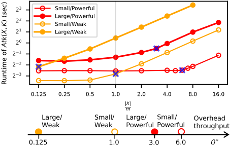
Fig. 1 plots the runtime of the attack function Atk(X,K) vs the data size |X| m with K = 10 and batch size m = 128 for the above four model/GPU setups. As |X| m increases initially, the runtime has little change because the GPU is underutilized for the small sized X and the runtime is dominated by an fixed overhead time associated with each Atk(X, K) call. This overhead time includes kernel launch overhead, memory allocation overhead, synchronization overhead, etc [Cook, 2012]. After |X| m reaches a certain size, marked by a blue cross, the runtime increases proportionally with |X| m .
Overhead Throughput. In this paper, overhead throughput, denoted by O∗ , refers to the maximum |X| m for the batch size m such that the runtime of Atk(X,K) is dominated by the overhead time. O∗ , which depends on the model/GPU setup, measures the maximum amount of data X that allows Atk(X,K) to run within the overhead time. A larger overhead throughput means that the GPU can process more data X within its fixed overhead time, thus, O∗ measures quantitatively how powerful a GPU is relative to the model (or how small a model is relative to the GPU). We say that Atk(X, K) is overhead dominated if |X| m ≤ O∗ , or is computation dominated if |X| m > O∗ . Importantly, increasing or decreasing the data X for overhead dominated Atk(X,K) does not significantly affect its runtime.
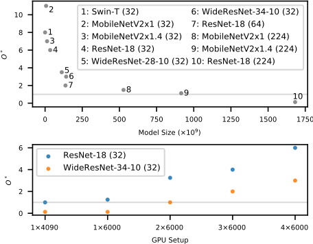
Returning to Fig. 1, Small/Powerful has the largest overhead throughput O∗ = 6.0, followed by 3.0 for Large/Powerful, 1.0 for Small/Weak, and 0.125 for Large/Weak. This makes sense because a powerful GPU requires a longer initialization time and a smaller model requires less time for model forward and backward propagation. Fig. 2 shows the values of O∗ for more model/GPU setups. Based on Fig. 1 and 2 and the above discussion, we summarize the following observations about O∗ .
Observations. (O1) Atk(X,K) can run with O∗ minibatches of data X within the overhead time, which provides the speedup of O∗ for attack generation compared to one minibatch at a time. For example, in Upper of Fig. 2, the models numbered 1 to 7 have O∗ ≥ 2, so Atk(X, K) can run within the overhead time for X of at least two minibatches of data. (O2) Each of the following leads to a larger O∗ : a powerful GPU, a small model, and a small batch size m. (O3) O∗ is independent of the distribution of training data because the work involved in K rounds of model forward and backward propagation depends only on the model size. (O4) Fig. 1 suggests a practical algorithm for finding the overhead throughput O∗ for a given model/GPU setup and the batch size m: plot the runtime vs |X| m by running Atk(X,K) with dummy examples X with |X| m increasing at some interval size, and O∗ is the |X| m value when the runtime starts to increase faster. Note that the choice of this value is not necessarily unique because it depends on the interpretation of "starts to increase faster".
Targeted Applications. According to observations O1 and O2 above, a large O∗ exists when GPU is powerful relative to the model size and when the batch size m is small. Several application scenarios meet these conditions. The first scenario is on-device model deployment where the model size is constrained by the limited memory and battery of mobile devices, e.g., MobileNets [Howard, 2017], but the model can be trained on powerful GPUs available at a cloud. Second, an organization (such as cloud computing) often invests in powerful GPUs to deal with various ML tasks from small models to large ones, and running powerful GPUs on small models leads to under-utilization of GPU, thus, a large O∗ . Note that "powerful" GPUs and "small" models are relative: a large model in an usual sense can be a "small" model to very powerful GPUs. Third, according to [Gorishniy et al., 2021; Asuncion et al., 2007], a small model with <1M parameters is sufficient for tabular data. While the acceleration of AT is motivated for expensive training, it is also important for time sensitive applications (like streaming data) where the model must be updated frequently in real time.
Our work does not intend to target at these applications: large vision or language models that are pre-trained once; large models that have a small O∗ , thus, computation dominated Atk(X,K), like those below the dotted line in Fig. 2; data are ample and a large batch size m is preferred, leading to a small O∗ . For example, by utilizing a large amount of generated images, the models in RobustBench [Croce et al., 2021] afford to use large batch size and large model size, at the expense of runtime. For tabular data, however, generated data tend to have a poor quality [Borisov et al., 2022].
3 Proposed Approach
By the notion of overhead throughput, if |X| m ≤ O∗ , Atk(X,K) incurs only the overhead time, where m is the batch size. For a large O∗ , we can read X from b minibatches X1, · · · ,Xb such that |X1|+···+|Xb| m ≤ O∗ , and run Atk(X1 ∪ · · · ∪ Xb,K) within the overhead time. In other words, we pack b minibatches into one attack function call without significantly increasing runtime. The number of minibatches packed, b, can be further increased when the base AT, such as BulletTrain [Hua et al., 2021], considers only a subset of influential examples from each minibatch for attack generation. Below, we present this approach, called AttackRider, followed by discussion and analysis of its speedup.
3.1 AttackRider-e
Alg. 1 presents AttackRider-e parameterized by the packing size e with e ≤ O∗ , where the condition e ≤ O∗ ensures that
Algorithm 1 AttackRider-e
Input: Training dataset D; Base AT BaseAT = {GetFB(·), Atk2(·), Upd(·)}; Packing size e
Output: Robust model fθ
1: Initialize f with random parameters fθ ← θ 2: repeat // Attack Generation: 3: FB ←GetFB(·) 4: b ← ⌈e/FB⌉ 5: Read b minibatches X fromD 6: ¯X ← Atk2(X, FB, fθ) // Model Update: 7: ¯X ← Shuff le( ¯X) 8: { ¯Xi, |i = 1, · · · , b} ←Divide( ¯X) 9: {Xi, |i = 1, · · · , b, examples in X correspond to ¯Xi} 10: for i = 1, · · · , b do 11: θ ← Upd( ¯Xi, Xi, fθ) 12: until training converged 13: return fθthe attack function Atk is run within the overhead time. We will discuss the choice of e shortly. To present AttackRider as a general acceleration approach that can be applied to an existing base AT that generates adversarial examples for one minibatch at a time, AttackRider has two inputs, the training dataset D as usual and a base AT denoted by BaseAT captured by three functions {GetFB(·),Atk2(·),Upd(·)}: the function for determining the percentage of examples in a minibatch for attack generation, the attack generation function, and the model update function, respectively. Examples of existing base ATs include BulletTrain, DBAC, PGDAT, TRADES, N-FGSM, or TDAT. Alg. 1 has two main steps, Attack Generation and Model Update, in each iteration.
Attack Generation. First, AttackRider calls GetFB(·) to obtain the fraction of examples, FB ≤ 1, for attack generation (line 3), reads b minibatches X (lines 4, 5), calls Atk2(X, FB, fθ) to generate adversarial examples for XB representing FB percentage of influential examples from X (i.e., |XB| |X| = FB) through running Atk(XB,K), and returns ¯X that contains the adversarial examples and the natural examples from X -XB. Note that |X| = b ×m, where m is the batch size of the base AT, and
We have
The choice of ceiling for computing b could lead to |XB| m slightly larger than e, thus, slightly larger than O∗ if e = O∗ . For simplicity, however, we continue to say that the condition e ≤ O∗ ensures that Atk(XB, K) is overhead dominated and incurs only the overhead time. By considering only influential examples XB with FB < 1, we have b > e and can pack more minibatches even for a small e. For example, the typical fraction of boundary examples in BulletTrain is about FB = 30%. With e = 1 and e = 2, we can pack b = ⌈1/0.3⌉ = 4 and b = ⌈2/0.3⌉ = 7 minibatches into one call of Atk, respectively.
GetFB(·) and Atk2(·) should be instantiated for the individual base AT. For GetFB(·), BulletTrain computes FB as the fraction of boundary examples based on the current classifier fθ; DBAC [Jung et al., 2023] computes FB using an attack ratio scheduling; PGDAT, TRADES, N-FGSM and TDAT have FB = 100%. For Atk2(X, FB, fθ), BulletTrain runs Atk(XB, K) for boundary examples XB such that |XB | |X| = FB (and optional Atk(XR,KR) for robust examples XR with KR ≪ K, which has a much smaller runtime than Atk(XB,K)); DBAC runs Atk(XB,K) for randomly selected examples XB fromX with |XB| |X| = FB; For PGDAT, TRADES, N-FGSM and TDAT, FB = 100% and Atk2(·) is simply Atk(XB, K) with XB = X.
Model Update. A straightforward model update is updating the model in one step using all b × m examples in ¯X. This essentially changes the original batch size m of the base AT to b × m, which would lead to a less frequent model update and poor generalization [Smith, 2018; Keskar et al., 2017]. To stick to the original batch size m of the base AT, we randomly shuffle the examples in ¯X (line 7) and divide evenly ¯X into b minibatches (line 8). The shuffling redistributes the adversarial examples evenly among the minibatches, allowing the model to generalize well [Neyshabur et al., 2017]. Upd( ¯Xi,Xi, fθ) adopts the base AT's loss and updates the model parameters θ, where Xi contains the natural examples corresponding to the examples in ¯Xi. For example, BulletTrain and DBAC can adopt PGDAT's loss on ¯Xi or TRADES's combined losses on ¯Xi and Xi, N-FGSM adopts PGDAT's loss, and TDAT has its own weighted loss similar to TRADES's loss.
3.2 Choosing e
A remaining question is how to choose the packing size e for AttackRider-e, where e ≤ O∗ . A larger e leads to a larger number b (Eq. (1)) of minibatches packed into one overhead dominated attack function call, thus, more time reduction. On the other hand, a larger b causes outdated adversarial examples because the adversarial examples in ¯X are generated based on the same model parameters θt (line 6) and are used to update the model parameters b times, i.e., θt+1, θt+2, · · · , θt+b (line 10, 11). These adversarial examples are outdated to different extents for updating θt+2, · · · , θt+b. However, model robustness can still be preserved with moderately outdated adversarial examples. This has to do with the adversarial example transferability [Wu et al., 2018] and training example diversity [Gong et al., 2019]. This transferability means that adversarial examples generated based on a substitute model can attack a similar target model [Wu et al., 2018], and in our context, it takes the form that outdated adversarial examples remain adversarial to subsequent updated models. Moreover, the model robustness could benefit from a more diverse set of training adversarial examples that have different extents of outdatedness. Our experiments show that small values e ∈ {1, 2} often achieve a good balance between speedup and accuracy for BulletTrain as the base AT, and e = O∗ often achieves a good balance between speedup and accuracy for other base ATs. More details are found in Sec. 3.3 and Sec. 4.1.
3.3 Analysis of Speedup
We analyze the speedup provided by AttackRider-e relative to the base AT, defined as the ratio of the runtime of the base AT over the runtime of AttackRider-e applied to the base AT. We consider a single iteration of AttackRider-e for processing b minibatches. AttackRider-e needs to run Atk(XB,K) once for b minibatches XB and Atk(XB,K) is overhead dominated. The base AT needs to run Atk(Xm,K) b times, each time on one minibatch Xm. With O∗ ≥ 1, which holds in most cases, Atk(Xm,K) is overhead dominated. Therefore, the runtimes of both Atk(XB, K) and Atk(Xm, K) are dominated by the fixed overhead time of attack function, denoted by T Atk . Let T Upd denote the model update time for one minibatch. Then the speedup of AttackRider-e in one iteration is equal to
where σ = T Atk /T Upd . rSpd can be extended to multiple iterations of AttackRider by replacing FB with its average value across the iterations in Eq. (3).
For a fixed e, a larger σ and a smaller FB lead to a larger rSpd. σ and FB are base AT specific, as follows. To estimate σ, we approximate T Atk /T Upd by the number of gradient descent steps performed during attack generation and model update. For PGDAT and TRADES, σ is K/1 and K/2, respectively, where K = 10 is the common setting, and FB = 100%; for BulletTrain with PGDAT's loss and TRADES's loss, denoted as BulletPGDAT and BulletTRADES, σ is the same as for PGDAT and TRADES, and FB ∈ [20%, 40%] [Hua et al., 2021]; for DBAC with N = 1 (i.e., reading one minibatch per attack generation call), σ is the same as for PGDAT and FB ∈ [50%, 100%] [Jung et al., 2023]; for N-FGSM and TDAT, σ is 1 1 and 12 , respectively, and FB = 100%.
With the above settings, BulletPGDAT permitting the largest rSpd and TDAT permitting the smallest rSpd. For example, with σ = K/1 and FB ≈ 40%, BulletPGDAT permits rSpd = ⌈e/0.4⌉×K+⌈e/0.4⌉ K+⌈e/0.4⌉ , which is 3.67 for K = 10 and e = 2; even the smallest rSpd for TDAT is 1.5e e+0.5 , which is at least 1 (because e ≥ 1 commonly holds). The empirical studies in Sec. 4.1 suggest a small e value for BulletPGDAT and BulletTRADES, to avoid excessive outdateness of adversarial examples, and e = O∗ for other base ATs to have a large speedup.
4 Experiments
We conduct extensive experiments to study the speedup provided by AttackRider for the targeted application scenarios discussed in Sec. 2. All experiments are conducted on a server with four NVIDIA RTX 6000 Ada GPUs and five datasets from image and tabular domains. Table 1 summarizes the GPUs, datasets, model information, batch size, and O∗ . We adopt ResNet-18 (RN) [He et al., 2016] for the image datasets and FT-Transformer (FT-T) [Gorishniy et al., 2021] for the tabular datasets. With our GPU server, these models represent varied extent of under-utilization of GPU indicated by the different O∗ values. The source code of AttackRider is available at at https://github.com/zxzhan/AttackRider.
| GPU | 4 × RTX 6000 | ||||
|---|---|---|---|---|---|
| Dataset | Image | Tabluar | |||
| CIFAR-10 | CIFAR-100 | TinyImageNet | Jannis | CoverType | |
| Model | RN | RN | RN | FT-T | FT-T |
| Input Size | 32×32×3 | 32×32×3 | 64×64×3 | 59 | 59 |
| Model Size | 34×109 | 34 × 109 | 137 × 109 | 9×10⁵ | 9×10⁵ |
| # Class | 10 | 100 | 200 | 4 | 7 |
| # Train | 50,000 | 50,000 | 100,000 | 53,588 | 371,847 |
| # Test | 10,000 | 10,000 | 10,000 | 16,749 | 116,203 |
| m | 128 | 128 | 128 | 512 | 1024 |
| O∗ | 6.0 | 6.0 | 2.0 | 6.0 | 3.0 |
Base ATs for AttackRider. We consider the seven base ATs discussed in Sec. 3.3 to which AttackRider is applied: the multi attack-step BulletPGDAT, BulletTRADES, DBAC, PGDAT, TRADES, with the attack step K = 10 following [Hua et al., 2021], and the single attack-step N-FGSM and TDAT. Since N-FGSM and TDAT are shown to outperform previous algorithms [Tong et al., 2024], we do not include older methods such as [Shafahi et al., 2019; Wong et al., 2020; Zhang et al., 2019a; Zheng et al., 2020; Ye et al., 2021]. DBAC can generate attacks for N ≥ 1 minibatches at a time. DBACN=1 serves as a base AT for AttackRider and DBACN=5 serves as a baseline to compare with AttackRider, where N = 5 was suggested in [Jung et al., 2023].
Evaluation Metrics. For each base AT, we evaluate speedup, clean accuracy (denoted by Clean), and robust accuracy before and after applying AttackRider to the base AT. We define the speedup Spd of AT algorithm A′ relative to AT algorithm A as the ratio t/t′ where t and t′ are the wall-clock training times of A and A′ . In particular, we are interested in the case that A and A′ are before and after applying AttackRider to a base AT, respectively. Note that Spd is the actual speedup, which is different from the estimated speedup rSpd in Sec. 3.3. The robust accuracy is measured by PGD20 and AutoAttack (AA) for image datasets and by PGD20 and PGD100 for tabular datasets (AutoAttack is not applicable to tabular data).
All models on the image datasets are trained with an SGD optimizer for 120 epochs following [Li et al., 2023a], and all models on the tabular datasets are trained with an AdamW optimizer for 100 epochs following [Gorishniy et al., 2021]. We evaluate the model that has the best test PGD20 robust accuracy within the specified number of epochs. For hyperparameter and base AT specific settings, we mostly follow the original papers of each base AT. The interested reader please refer to the separate Appendix file for more details.
Sec. 4.1 investigates and suggests the choice of e for AttackRider-e. Sec. 4.2 presents the main results on the effectiveness of AttackRider-e in terms of our evaluation metrics. Sec. 4.3 studies the effectiveness of the Shuffle and Divide functions of AttackRider-e.
| Clean | PGD20 | AA | rSpd | Spd | ¯b | Time | |
|---|---|---|---|---|---|---|---|
| BulletPGDAT | 86.56 | 49.28 | 45.58 | - | 1.00 | 1.0 | 173 |
| + AR-1 | 86.32 | 49.20 | 45.21 | 2.54 | 1.96 | 3.0 | 88 |
| + AR-2 | 86.48 | 49.15 | 45.01 | 3.81 | 2.98 | 5.3 | 58 |
| + AR-3 | 86.72 | 48.25 | 44.86 | 4.75 | 3.60 | 7.6 | 48 |
| + AR-4 | 86.65 | 48.15 | 44.60 | 5.39 | 3.93 | 9.6 | 44 |
| + AR-5 | 86.50 | 47.35 | 44.31 | 5.91 | 4.32 | 11.6 | 40 |
| + AR-6 (O∗ | 86.48 | 47.90 | 44.08 | 6.34 | 4.55 | 13.6 | 38 |
| ) BulletTRADES | 82.79 | 52.38 | 48.82 | - | 1.00 | 1.0 | 213 |
| + AR-1 | 82.54 | 52.18 | 48.55 | 2.74 | 2.52 | 4.2 | 85 |
| + AR-2 | 82.63 | 52.20 | 48.50 | 3.73 | 3.45 | 8.2 | 62 |
| + AR-3 | 81.93 | 52.00 | 47.96 | 4.19 | 3.80 | 11.6 | 56 |
| + AR-4 | 81.62 | 51.65 | 47.39 | 4.52 | 4.02 | 15.3 | 53 |
| + AR-5 | 81.69 | 52.00 | 47.33 | 4.73 | 4.18 | 18.7 | 51 |
| + AR-6 (O∗ ) | 81.63 | 51.14 | 47.27 | 4.90 | 4.26 | 22.3 | 50 |
| DBACN=1 | 85.33 | 49.64 | 46.32 | - | 1.00 | 1.0 | 167 |
| + AR-1 | 85.32 | 49.54 | 46.62 | 1.76 | 1.44 | 1.9 | 116 |
| + AR-2 | 85.83 | 48.79 | 45.89 | 2.67 | 2.45 | 3.2 | 68 |
| + AR-3 | 85.16 | 49.02 | 45.78 | 3.43 | 2.99 | 4.5 | 56 |
| + AR-4 | 84.98 | 49.56 | 46.37 | 4.07 | 3.52 | 5.9 | 48 |
| + AR-5 | 84.78 | 49.36 | 46.10 | 4.61 | 3.80 | 7.2 | 44 |
| + AR-6 (O∗ ) | 85.36 | 49.05 | 46.15 | 5.08 | 4.08 | 8.6 | 41 |
| DBACN=5 | 85.37 | 49.27 | 46.36 | - | 3.31 | 5.0 | 51 |
| PGDAT | 84.76 | 49.95 | 46.72 | - | 1.00 | 1.0 | 162 |
| + AR-1 | 84.76 | 49.95 | 46.72 | 1.00 | 1.00 | 1.0 | 162 |
| + AR-2 | 84.16 | 50.12 | 46.75 | 1.83 | 1.77 | 2.0 | 92 |
| + AR-3 | 83.92 | 50.54 | 46.93 | 2.54 | 2.33 | 3.0 | 70 |
| + AR-4 | 84.01 | 50.13 | 46.80 | 3.14 | 2.80 | 4.0 | 58 |
| + AR-5 | 83.89 | 50.10 | 46.95 | 3.67 | 3.15 | 5.0 | 52 |
| + AR-6 (O∗ ) | 83.99 | 50.07 | 46.77 | 4.13 | 3.42 | 6.0 | 47 |
| TRADES | 81.14 | 52.53 | 48.72 | - | 1.00 | 1.0 | 185 |
| + AR-1 | 81.14 | 52.53 | 48.72 | 1.00 | 1.00 | 1.0 | 185 |
| + AR-2 | 82.47 | 53.19 | 49.77 | 1.71 | 1.59 | 2.0 | 116 |
| + AR-3 | 82.05 | 52.79 | 49.21 | 2.25 | 2.08 | 3.0 | 89 |
| + AR-4 | 81.99 | 52.55 | 49.17 | 2.67 | 2.42 | 4.0 | 77 |
| + AR-5 | 82.15 | 52.57 | 49.18 | 3.00 | 2.70 | 5.0 | 69 |
| + AR-6 (O∗ ) | 82.59 | 52.26 | 48.82 | 3.27 | 2.86 | 6.0 | 65 |
| N-FGSM | 83.59 | 46.53 | 43.60 | - | 1.00 | 1.0 | 36 |
| + AR-1 | 83.59 | 46.53 | 43.60 | 1.00 | 1.00 | 1.0 | 36 |
| + AR-2 | 83.04 | 46.41 | 43.96 | 1.33 | 1.22 | 2.0 | 29 |
| + AR-3 | 83.28 | 46.16 | 43.63 | 1.50 | 1.35 | 3.0 | 27 |
| + AR-4 | 83.12 | 46.87 | 43.85 | 1.60 | 1.41 | 4.0 | 26 |
| + AR-5 | 82.53 | 46.25 | 43.87 | 1.67 | 1.47 | 5.0 | 24 |
| + AR-6 (O∗ ) | 83.67 | 45.65 | 43.29 | 1.71 | 1.50 | 6.0 | 24 |
| TDAT | 83.17 | 53.76 | 46.81 | - | 1.00 | 1.0 | 58 |
| + AR-1 | 83.17 | 53.76 | 46.81 | 1.00 | 1.00 | 1.0 | 58 |
| + AR-2 | 83.06 | 53.46 | 46.87 | 1.20 | 2.0 | 48 | |
| + AR-3 | 84.03 | 53.92 | 47.04 | 1.29 | 1.22 | 3.0 | 45 |
| + AR-4 | 82.70 | 53.40 | 46.49 | 1.33 | 1.29 1.33 | 4.0 | 44 |
| + AR-5 | 81.30 | 52.97 | 46.24 | 1.36 | 1.35 | 5.0 | 43 |
| + AR-6 (O∗ ) | 83.41 | 53.05 | 46.51 | 1.38 | 1.40 | 6.0 | 42 |
4.1 Sensitivity of Packing Size e
To provide the guideline for choosing e of AttackRider-e, we first study the sensitivity of e using CIFAR-10 dataset on the RN model. The results are reported in Table 2. Each base AT is color coded and represented by the first row in that color, followed by the "+ AR-e" rows that represent AttackRider-e applied to the base AT. We also include DBACN=5 for comparison with AttackRider. Spd and rSpd are relative to each individual base AT (i.e., the first row of each color), therefore, are not comparable across different base ATs.
In general, a larger e provides more Spd but also more drop in accuracies. The accuracy drop is due to the adversarial example outdatedness discussed in Sec. 3.2. With BulletTrain (BulletPGDAT and BulletTRADES) as the base AT, a small e ∈ {1, 2}, indicated in boldface, is able to provide a good trade-off between speedup and accuracies compared to the base AT. For example, applying AR-2 provides Spd of 2.98 and 3.45 relative to the base AT BullletPGDAT and BullletTRADES while keeping the change of PGD20 and AA within 1%. This is because BulletTrain considers about FB ∈ [20%, 40%] boundary examples for attack generation, allowing AttackRider-e to pack more minibatches in each attack generation even for a small e, as seen from ¯b much larger than e.
DBACN=1 generates attacks for about FB ∈ [50%, 100%] examples in a minibatch, and PGDAT, TRADES, N-FGSM and TDAT generate attacks for all examples, i.e., FB = 100%. In these cases, AttackRider-e packs fewer minibatches for each attack generation, leading to a smaller Spd. In addition, the single attack-step N-FGSM and TDAT have a less expensive attack function, which further limits the time reduction of AttackRider. For these base ATs, a large e = 6 (i.e., O∗ ), marked in boldface, is needed to provide a speedup. We did not consider AttackRider-e with e > O∗ be-
cause such an AttackRider-e becomes computation dominated, thus, does not provide further speedup compared to AttackRider-O∗ . Finally, rSpd is generally larger than Spd because we estimate the ratio T Atk /T Upd by K/1 (or K/2) in Eq. (3) for a K-attack step AT, but the actual wall-clock ratio should be (K+c1)/(1+c2) (or (K+c1)/(2+c2)) for some fixed costs c1 and c2. For single-attack step N-FGSM and TDAT, the extent of overestimation is less so that rSpd is closer to Spd.
In summary, we recommend e ∈ {1, 2} when applying AttackRider-e to BulletTrain and recommend e = O∗ when applying AttackRider-e to DBACN=1, PGDAT, TRADES, NFGSM, and TDAT.
4.2 Main Results
We now evaluate AttackRider-e using all datasets. Following the study in Sec. 4.1, we consider e ∈ {1, 2} for applying AttackRider-e to BulletTrain and consider e = O∗ for applying AttackRider-e to the other base ATs, i.e., DBACN=1, PGDAT, TRADES, N-FGSM and TDAT.
Image Datasets (Table 3). The results on CIFAR-10 have been reported and analyzed in Sec. 4.1. Here, we report the results on CIFAR-100 and TinyImageNet in Table 3. For the base AT BulletTrain, applying AR-2 provides a good tradeoff between speedup and accuracies, and for the other base ATs, applying AR-O∗ , where O∗ = 6 on CIFAR-100 and O∗ = 2 on TinyImageNet, provides a good trade-off between speedup Spd and accuracies. For most base ATs, Spd is more than 3, and for the single attack-step N-FGSM and TDAT, Spd is around 1.5.
| Clean | PGD20 | AA | rSpd | Spd | ¯b | Time | |
|---|---|---|---|---|---|---|---|
| BulletPGDAT | 63.34 | 24.90 | 22.22 | - | 1.00 | 1.0 | 206 |
| + AR-1 | 63.42 | 24.75 | 21.90 | 2.51 | 2.05 | 3.0 | 101 |
| + AR-2 | 63.85 | 24.42 | 21.73 | 3.82 | 3.50 | 5.3 | 59 |
| BulletTRADES | 58.64 | 29.61 | 24.74 | - | 1.00 | 1.0 | 246 |
| + AR-1 | 58.67 | 29.58 | 24.72 | 2.96 | 2.80 | 4.9 | 88 |
| + AR-2 | 58.21 | 29.32 | 24.21 | 3.92 | 3.63 | 9.4 | 68 |
| DBACN=1 | 59.35 | 27.89 | 24.26 | - | 1.00 | 1.0 | 167 |
| + AR-6 (O∗ ) | 58.91 | 27.06 | 23.43 | 5.09 | 3.71 | 8.6 | 45 |
| CIFAR-100 DBACN=5 | 59.43 | 27.55 | 23.98 | - | 3.27 | 5.0 | 51 |
| PGDAT | 57.28 | 28.54 | 24.62 | - | 1.00 | 1.0 | 166 |
| + AR-6 (O∗ ) | 57.32 | 27.84 | 23.92 | 4.13 | 3.48 | 6.0 | 48 |
| TRADES | 58.10 | 29.59 | 25.13 | - | 1.00 | 1.0 | 193 |
| + AR-6 (O∗ ) | 58.23 | 29.55 | 24.52 | 3.27 | 2.99 | 6.0 | 65 |
| N-FGSM | 55.15 | 26.86 | 23.15 | - | 1.00 | 1.0 | 38 |
| + AR-6 (O∗ ) | 56.69 | 26.44 | 22.81 | 1.71 | 1.57 | 6.0 | 24 |
| TDAT | 58.39 | 31.31 | 24.26 | - | 1.00 | 1.0 | 60 |
| + AR-6 (O∗ ) | 57.51 | 30.89 | 23.82 | 1.38 | 1.45 | 6.0 | 41 |
| BulletPGDAT | 49.81 | 15.10 | 12.52 | - | 1.00 | 1.0 | 431 |
| + AR-1 | 50.18 | 14.52 | 12.10 | 2.73 | 2.44 | 3.3 | 177 |
| + AR-2 (O∗ ) | 50.34 | 14.49 | 12.03 | 4.16 | 2.82 | 6.1 | 153 |
| BulletTRADES | 45.40 | 18.22 | 13.98 | - | 1.00 | 1.0 | 521 |
| + AR-1 | 45.43 | 18.20 | 13.60 | 2.88 | 2.96 | 4.6 | 176 |
| + AR-2 (O∗ ) | 45.61 | 18.09 | 13.47 | 3.87 | 3.45 | 9.1 | 151 |
| DBACN=1 | 47.23 | 19.10 | 15.28 | - | 1.00 | 1.0 | 349 |
| Tiny + AR-2 (O∗ ) | 47.65 | 18.49 | 15.11 | 2.67 | 1.79 | 3.2 | 195 |
| ImageNet DBACN=5 | 47.06 | 18.32 | 14.39 | - | 1.78 | 5.0 | 196 |
| PGDAT | 45.52 | 19.83 | 16.15 | - | 1.00 | 1.0 | 340 |
| + AR-2 (O∗ ) | 45.40 | 19.75 | 15.90 | 1.83 | 1.49 | 2.0 | 228 |
| TRADES | 43.26 | 19.45 | 14.52 | - | 1.00 | 1.0 | 417 |
| + AR-2 (O∗ ) | 42.95 | 19.32 | 14.34 | 1.71 | 1.53 | 2.0 | 272 |
| N-FGSM | 46.50 | 18.57 | 15.17 | - | 1.00 | 1.0 | 81 |
| + AR-2 (O∗ ) | 46.40 | 18.46 | 15.07 | 1.33 | 1.46 | 2.0 | 56 |
| TDAT | 42.89 | 22.61 | 15.26 | - | 1.00 | 1.0 | 135 |
| + AR-2 (O∗ ) | 44.19 | 22.77 | 15.33 | 1.20 | 1.23 | 2.0 | 110 |
| Clean | PGD20 | PGD100 | rSpd | Spd | ¯b | Time | ||
|---|---|---|---|---|---|---|---|---|
| Jannis | BulletPGDAT | 65.87 | 54.76 | 54.78 | - | 1.00 | 1.0 | 42 |
| + AR-1 | 65.13 | 55.15 | 55.14 | 2.55 | 2.56 | 3.0 | 16 | |
| + AR-2 | 65.55 | 54.36 | 54.41 | 3.91 | 3.77 | 5.5 | 11 | |
| DBACN=1 | 65.37 | 54.92 | 54.92 | - | 1.00 | 1.0 | 30 | |
| + AR-6 (O∗ ) | 64.20 | 54.39 | 54.40 | 4.97 | 3.20 | 8.2 | 9 | |
| DBACN=5 | 64.77 | 54.79 | 54.80 | - | 2.61 | 5.0 | 11 | |
| PGDAT | 64.80 | 55.14 | 55.14 | - | 1.00 | 1.0 | 29 | |
| + AR-6 (O∗ ) | 63.61 | 55.06 | 55.02 | 4.13 | 2.56 | 6.0 | 11 | |
| BulletPGDAT | 88.56 | 74.20 | 73.82 | - | 1.00 | 1.0 | 151 | |
| + AR-1 | 88.87 | 73.91 | 73.63 | 3.19 | 3.22 | 4.1 | 47 | |
| + AR-2 | 88.55 | 73.99 | 73.73 | 4.67 | 3.79 | 7.4 | 40 | |
| Cover Type | DBACN=1 | 86.06 | 75.35 | 75.11 | - | 1.00 | 1.0 | 122 |
| + AR-3 (O∗ ) | 86.21 | 75.46 | 75.25 | 3.34 | 2.25 | 4.4 | 54 | |
| DBACN=5 | 85.89 | 75.18 | 75.01 | - | 2.17 | 5.0 | 56 | |
| PGDAT | 85.55 | 75.53 | 75.33 | - | 1.00 | 1.0 | 120 | |
| + AR-3 (O∗ ) | 85.22 | 75.40 | 75.21 | 2.54 | 1.77 | 3.0 | 68 |
Second, on CIAFR-10 and CIFAR-100 that have the larger O∗ = 6, applying AR-O∗ to DBACN=1 achieves more speedup than DBACN=5. On TinyImageNet that has the smaller O∗ = 2, applying AR-O∗ to DBACN=1 achieves a similar speedup but better accuracy compared to DBACN=5.
Third, in the case of O∗ > 1 as in our experiments, reducing the data X (by considering a subset of minibatch) for attack generation Atk(X,K) fails to reduce time. This is demonstrated by the observation that PGDAT incurs less time than BulletPGDAT and DBACN=1, TRADES incurs less time than BulletTRADES. As matter of fact, the opposite is true when O∗ > 1, that is, packing more data X, up to O∗ minibatches, in the attack generation, can reduce time. This is exactly the approach of AttackRider.
Tabular Datasets (Table 4). ℓ2-bounded robustness was suggested for tabular datasets [Ballet et al., 2019], making NFGSM and TDAT that adopt the ℓ∞-bounded FGSM attack inapplicable [Dolatabadi et al., 2022]. In addition, we observed that TRADES performs worse than PGDAT on tabular data. Therefore, we consider only applying AttackRider-e to BulletPGDAT, DBACN=1 and PGDAT in Table 4. Similar to those in Table 3, AttackRider-e can effectively provide speedups while obtaining comparable accuracy with these base ATs.
| Clean | PGD20 | AA | Time | |
|---|---|---|---|---|
| BulletPGDAT + AR-2 | 86.48 | 49.15 | 45.01 | 58 |
| w/o Shuffle | 84.52 | 48.90 | 43.23 | 59 |
| w/o Divide | 83.97 | 44.80 | 41.03 | 43 |
| BulletTRADES + AR-2 | 82.63 | 52.20 | 48.50 | 62 |
| w/o Shuffle | 76.45 | 47.65 | 43.52 | 65 |
| w/o Divide | 77.14 | 47.55 | 42.64 | 47 |
| DBACN=1 + AR-6 | 85.36 | 49.05 | 46.15 | 41 |
| w/o Shuffle | 85.37 | 48.91 | 46.04 | 41 |
| w/o Divide | 81.78 | 44.44 | 41.50 | 26 |
| PGDAT + AR-6 | 83.99 | 50.07 | 46.77 | 47 |
| w/o Shuffle | 83.27 | 49.65 | 46.54 | 47 |
| w/o Divide | 82.43 | 45.70 | 42.58 | 32 |
| TRADES + AR-6 | 82.59 | 52.26 | 48.82 | 65 |
| w/o Shuffle | 81.65 | 52.23 | 48.46 | 65 |
| w/o Divide | 78.98 | 49.28 | 45.49 | 38 |
| N-FGSM + AR-6 | 83.67 | 45.65 | 43.29 | 24 |
| w/o Shuffle | 83.14 | 45.89 | 43.31 | 25 |
| w/o Divide | 81.37 | 40.78 | 38.54 | 14 |
| TDAT + AR-6 | 83.41 | 53.05 | 46.51 | 42 |
| w/o Shuffle | 83.08 | 53.73 | 46.89 | 42 |
| w/o Divide | 78.44 | 48.81 | 42.31 | 14 |
4.3 Ablation Studies
AttackRider-e employs the Shuffle and Divide functions to eliminate the bias of a minibatch for updating the model at the original batch size. To study the contribution of these functions, we examine the options of turning off these functions. "w/o Shuffle" denotes no Shuffling function performed and "w/o Divide" denotes no Divide function performed (i.e., updating the model once using the data consisting of multiple minibatches). Table 5 compares AttackRider with these options. In general, there is a significant drop in clean accuracy and robust accuracy for "w/o Shuffle" and "w/o Divide". These findings showcase the importance of the Shuffle and Divide functions in AttackRider-e.
5 Conclusion
We proposed AttackRider to speed up adversarial training (AT) by exploiting GPUs that are under-utilized for attack generation for a small minibatch. To better utilize the GPU, we introduced the notion of overhead throughput to quantify the extent of GPU under-utilization and to guide us to pack multiple minibatches into a single attack generation call without increasing the time of each call. To our knowledge, this is the first work that formally quantifies the extent of GPU under-utilization for AT speedup. We presented application scenarios that warrant a large overhead throughput for achieving a speedup. Evaluation using various under-utilization of GPU settings and datasets supports our claims.
Acknowledgments
This project was supported in part by collaborative research funding from the National Research Council of Canada's Artificial Intelligence for Logistics Program and in part by Ke Wang's discovery grant from Natural Sciences and Engineering Research Council of Canada.
@inproceedings{ijcai2025p774,
  title     = {Accelerating Adversarial Training on Under-Utilized GPU},
  author    = {Zhan, Zhuoxin and Wang, Ke and Xiong, Pulei},
  booktitle = {Proceedings of the Thirty-Fourth International Joint Conference on
               Artificial Intelligence, {IJCAI-25}},
  publisher = {International Joint Conferences on Artificial Intelligence Organization},
  editor    = {James Kwok},
  pages     = {6958--6966},
  year      = {2025},
  month     = {8},
  note      = {Main Track},
  doi       = {10.24963/ijcai.2025/774},
  url       = {https://doi.org/10.24963/ijcai.2025/774},
}
TY - CPAPER TI - Accelerating Adversarial Training on Under-Utilized GPU AU - Zhan, Zhuoxin AU - Wang, Ke AU - Xiong, Pulei T2 - Proceedings of the Thirty-Fourth International Joint Conference on Artificial Intelligence, IJCAI-25 PB - International Joint Conferences on Artificial Intelligence Organization PY - 2025 SP - 6958 EP - 6966 DO - 10.24963/ijcai.2025/774 UR - https://doi.org/10.24963/ijcai.2025/774 ER -Copied
Machine-readable versions of this paper, for tools and AI agents:





