
Fault Diagnosis in REDNet Model Space
Proceedings of the Thirty-Fourth International Joint Conference on Artificial Intelligence. Main Track. Pages 7209-7217.
https://doi.org/10.24963/ijcai.2025/802
Keywords
- Machine Learning: ML: Classification
- Data Mining: DM: Anomaly/outlier detection
- Machine Learning: ML: Representation learning
- Machine Learning: ML: Recurrent networks
Abstract
Fault Diagnosis (FD) in time-varying data presents considerations such as limited training data, intra- and inter-dimensional correlations, and constraints of training time. In response, this paper introduces FD in the Reservoir-Embedded-Directional Network (REDNet) model space. Model-oriented methods utilize well-fitted networks or functions, denoted as "models" that capture data's changing information, as more stable and parsimonious representations of the data. Our approach employs REDNet for data fitting, wherein multiple reservoirs are organized along intrinsic correlation directions to establish intra- and inter-dimensional dependencies, thereby capturing multi-directional dynamics in high-dimensional data.
Representing each data instance with an independently fitted REDNet model maps these instances into a class-separable REDNet model space, where FD could be performed on the models rather than the original data. Concentrating on the data-intrinsic dynamics, our method achieves rapid training speeds, and maintains robust performance even with minimal training data. Experiments on several datasets demonstrate its effectiveness.
- [Altman, 1992] Naomi S Altman. An introduction to ker- nel and nearest-neighbor nonparametric regression. The American Statistician, 46(3):175-185, 1992.
- [Chen et al., 2013a] Huanhuan Chen, Fengzhen Tang, Pe- ter Tino, and Xin Yao. Model-based kernel for efficient time series analysis. In Proceedings of the 19th ACM SIGKDD international conference on Knowledge discov- ery and data mining, pages 392-400, 2013.
- [Chen et al., 2013b] Huanhuan Chen, Peter Tiňo, Ali Rodan, and Xin Yao. Learning in the model space for cognitive fault diagnosis. IEEE transactions on neural networks and learning systems, 25(1):124-136, 2013.
- [Chen et al., 2020] Zhe Chen, Huimin Lu, Shiqing Tian, Junlin Qiu, Tohru Kamiya, Seiichi Serikawa, and Lizhong Xu. Construction of a hierarchical feature enhancement network and its application in fault recognition. IEEE Transactions on Industrial Informatics, 17(7):4827-4836, 2020.
- [Chen et al., 2024] Ao Chen, Xiren Zhou, Yizhan Fan, and Huanhuan Chen. Underground diagnosis based on gpr and learning in the model space. IEEE Transactions on Pat- tern Analysis and Machine Intelligence, 46(5):3832-3844, 2024.
- [Chiu and Minku, 2022] Chun Wai Chiu and Leandro L. Minku. A diversity framework for dealing with multiple types of concept drift based on clustering in the model space. IEEE Transactions on Neural Networks and Learn- ing Systems, 33(3):1299-1309, 2022.
- [Cho et al., 2014] Kyunghyun Cho, B van Merrienboer, Caglar Gulcehre, F Bougares, H Schwenk, and Yoshua Bengio. Learning phrase representations using rnn encoder-decoder for statistical machine translation. In Conference on Empirical Methods in Natural Language Processing (EMNLP 2014), 2014.
- [Cortes and Vapnik, 1995] Corinna Cortes and Vladimir Vapnik. Support-vector networks. Machine learning, 20(3):273-297, 1995.
- [Ghanbari et al., 2023] Navidreza Ghanbari, Yassin Riyazi, Farzad Shirazi, and Ahmad Kalhor. Enhanced gearbox fault diagnosis with fusion lstm-cnn network. In Interna- tional Conference on Acoustics and Vibrations, 12 2023.
- [Glowacz et al., 2021] Adam Glowacz, Ryszard Tadeusiewicz, Stanislaw Legutko, Wahyu Caesaren- dra, Muhammad Irfan, Hui Liu, Frantisek Brumercik, Miroslav Gutten, Maciej Sulowicz, Jose Alfonso An- tonino Daviu, et al. Fault diagnosis of angle grinders and electric impact drills using acoustic signals. Applied Acoustics, 179:108070, 2021.
- [Jaeger, 2001] Herbert Jaeger. The "echo state" approach to analysing and training recurrent neural networks-with an erratum note. Bonn, Germany: German National Re- search Center for Information Technology GMD Technical Report, 148(34):13, 2001.
- [Kumar et al., 2022] Dileep Kumar, Sanaullah Mehran, Muhammad Zakir Shaikh, Majid Hussain, Bhawani Shankar Chowdhry, and Tanweer Hussain. Triaxial bearing vibration dataset of induction motor under varying load conditions. Data in Brief, 42:108315, 2022.
- [Liu et al., 2021] Ze Liu, Yutong Lin, Yue Cao, Han Hu, Yixuan Wei, Zheng Zhang, Stephen Lin, and Baining Guo. Swin transformer: Hierarchical vision transformer using shifted windows. In Proceedings of the IEEE/CVF in- ternational conference on computer vision, pages 10012- 10022, 2021.
- [Loparo, 2012] KA Loparo. Case western reserve university bearing data center. Bearings Vibration Data Sets, Case Western Reserve University, pages 22-28, 2012.
- [Lukoševičius and Jaeger, 2009] Mantas Lukoševičius and Herbert Jaeger. Reservoir computing approaches to recur- rent neural network training. Computer science review, 3(3):127-149, 2009.
- [Ma et al., 2020] Qianli Ma, Sen Li, Wanqing Zhuang, Ji- abing Wang, and Delu Zeng. Self-supervised time series clustering with model-based dynamics. IEEE Transactions on Neural Networks and Learning Systems, 32(9):3942- 3955, 2020.
- [Quevedo et al., 2014] Joseba Quevedo, Huanhuan Chen, Miquel À Cugueró, Peter Tino, Vicenc ¸Puig, Diego Garciá, Ramon Sarrate, and Xin Yao. Combining learn- ing in model space fault diagnosis with data valida- tion/reconstruction: Application to the barcelona water network. Engineering Applications of Artificial Intelli- gence, 30:18-29, 2014.
- [Shao et al., 2019] Siyu Shao, Stephen McAleer, Ruqiang Yan, and Pierre Baldi. Highly accurate machine fault di- agnosis using deep transfer learning. IEEE Transactions on Industrial Informatics, 15(4):2446-2455, 2019.
- [Shi and Zhang, 2020] Qian Shi and Hui Zhang. Fault di- agnosis of an autonomous vehicle with an improved svm algorithm subject to unbalanced datasets. IEEE Transac- tions on Industrial Electronics, 68(7):6248-6256, 2020.
- [Srivastava et al., 2007] Prashant K Srivastava, Dhwani K Desai, Soumyadeep Nandi, and Andrew M Lynn. Hmm-mode-improved classification using profile hidden markov models by optimising the discrimination threshold and modifying emission probabilities with negative train- ing sequences. BMC bioinformatics, 8(1):1-17, 2007.
- [Su et al., 2019] Ya Su, Youjian Zhao, Chenhao Niu, Rong Liu, Wei Sun, and Dan Pei. Robust anomaly detection for multivariate time series through stochastic recurrent neu- ral network. In Proceedings of the 25th ACM SIGKDD international conference on knowledge discovery & data mining, pages 2828-2837, 2019.
- [Woo et al., 2023] Sanghyun Woo, Shoubhik Debnath, Ronghang Hu, Xinlei Chen, Zhuang Liu, In So Kweon, and Saining Xie. Convnext v2: Co-designing and scaling convnets with masked autoencoders. In Proceedings of the IEEE/CVF Conference on Computer Vision and Pattern Recognition, pages 16133-16142, 2023.
- [Wu et al., 2021] Haixu Wu, Jiehui Xu, Jianmin Wang, and Mingsheng Long. Autoformer: Decomposition transform- ers with auto-correlation for long-term series forecast- ing. Advances in neural information processing systems, 34:22419-22430, 2021.
- [Wu et al., 2022] Jiamin Wu, Xiren Zhou, and Qiuju Chen. A characteristic of speaker's audio in the model space based on adaptive frequency scaling. In 2022 8th Interna- tional Conference on Big Data and Information Analytics (BigDIA), pages 99-103. IEEE, 2022.
- [Wu et al., 2023] Haixu Wu, Tengge Hu, Yong Liu, Hang Zhou, Jianmin Wang, and Mingsheng Long. Timesnet: Temporal 2d-variation modeling for general time series analysis. Proceedings of the International Conference on Learning Representations, 2023.
- [Xiong and Yeung, 2002] Yimin Xiong and Dit-Yan Yeung. Mixtures of arma models for model-based time series clus- tering. In 2002 IEEE International Conference on Data Mining, 2002. Proceedings., pages 717-720. IEEE, 2002.
- [Zhao et al., 2017] Rui Zhao, Dongzhe Wang, Ruqiang Yan, Kezhi Mao, Fei Shen, and Jinjiang Wang. Machine health monitoring using local feature-based gated recurrent unit networks. IEEE Transactions on Industrial Electronics, 65(2):1539-1548, 2017.
- [Zhou et al., 2022] Tian Zhou, Ziqing Ma, Qingsong Wen, Xue Wang, Liang Sun, and Rong Jin. Fedformer: Fre- quency enhanced decomposed transformer for long-term series forecasting. In International Conference on Ma- chine Learning, pages 27268-27286. PMLR, 2022.
- [Zhou et al., 2023] Xiren Zhou, Shikang Liu, Ao Chen, Qi- uju Chen, Fang Xiong, Yumin Wang, and Huanhuan Chen. Underground anomaly detection in GPR data by learning in the c3 model space. IEEE Transactions on Geoscience and Remote Sensing, pages 1-11, 2023.
References were extracted automatically from the PDF and may contain errors.
Full text extracted automatically from the PDF; figures, tables and equations may differ. The PDF is the version of record.
1 Introduction
The development of sensors and data monitoring capabilities has facilitated the collection of sequential data in multidimensional formats, where each point includes multiple observations or variables, simultaneously capturing various aspects of a system or process. Fault Diagnosis (FD) from such data plays an increasingly important role in various fields. Typically, the FD process could be examined through two stages: 1) Fault detection, to ascertain the occurrence of a fault; and 2) Fault isolation, to identify the specific fault type. In practice, FD is often streamlined to determine whether a data instance represents a fault and, if so, identify its type.
Considerable efforts have been devoted to various types of FD tasks. A straightforward approach involves comparing newly collected data instances with the predictions of the underlying mathematical model that is constructed based on the "normal" system or data. However, the accuracy and availability of such underlying mathematical models in real-world data scenarios are questionable. Addressing this, researchers have explored the use of Machine Learning (ML) algorithms, such as the Bayesian classifier [Glowacz et al., 2021] and Support Vector Machine (SVM) [Shi and Zhang, 2020], accompanied by manual feature selections and advanced data or signal processing techniques. Additionally, Deep Learning (DL) methods, primarily based on Deep Neural Networks [Zhao et al., 2017; Shao et al., 2019], have been applied to FD tasks, due to their automated feature extraction abilities when dealing with complex data or systems. Yet, behind the effective usage of most DL methods, there exist two necessary assumptions: 1) Sufficient and diverse labeled data with consistent distributions between training and test sets; 2) Use of gradient-descent-based methods for training, demanding significant training time and computing resources.
∗Corresponding author: Huanhuan Chen.
In practical FD tasks, the following considerations should be noted: 1) Faults involve unknowns, such as abrupt changes or distributions, necessitating FD methods to work with limited training data; 2) Underlying environments are variable, even for similar tasks, making it challenging to ensure the effectiveness of an FD method trained for one environment in others; 3) Timeliness requirements demand a prompt FD launch upon data collection in a specific task.
In response to the above considerations, the concept of model-oriented learning has been introduced for real-time or on-site classification and diagnosis tasks. The core of model-oriented methods involves representing original data instances with functions or networks, often denoted as "models", which encapsulate the dynamics (i.e., the changing information) within the data. Consequently, classification algorithms could be applied to the models, usually the key parameters of the data-representing function or network, instead of the original data. Notably, this approach places a heightened emphasis on the data-intrinsic changing information, and often demands less training data and duration compared to DL techniques, especially coupled with an appropriate data-fitting approach for adequate dynamic encapsulation.
Nevertheless, for time-series data, existing model-oriented FD research typically utilizes the Echo State Network (ESN)- based approaches [Jaeger, 2001] for data fitting and representation, which fits the data along the data-collection order. In the case of complex systems and data, effective dynamics within the data may not be limited to any single direction. For example, when diagnosing mechanical or industrial faults, significant correlations exist both along the data-collection order (timeline) and synchronous measurements from various sensors (cross-dimensional). Relying solely on ESN for data fitting risks neglecting these multi-directional dynamics. Moreover, applying ESN to multi-dimensional data, or integrating multiple ESNs each fitted along different directions [Zhou et al., 2023], results in overly larger-size fitted models. This increase in model size and complexity poses challenges for subsequent model-oriented processing.
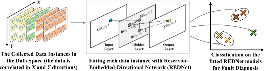
To address the above challenges of FD in high-dimensional time-series data, this paper introduces FD in the ReservoirEmbedded-Directional Network (REDNet) model space, as showcased in Figure 1. REDNet 1 denotes a reservoir computing network that incorporates multiple reservoirs in its hidden layer, each aligned with a distinct intrinsic correlation direction, ensuring a one-to-one correspondence between a reservoir and data-inherent directional dependencies. By establishing intricate connections between data points in multiple directions (within and among data dimensions), fitting data with REDNet accurately and comprehensively captures the data-inherent multi-directional dynamics. Since normal data instances share similar dynamic patterns, their corresponding fitted models tend to be alike. In contrast, fault data, characterized by distinct dynamic behaviors, yield fitted models that differ markedly from those of normal instances and from each other. Consequently, representing each data instance with an individually fitted model maps the original data instances into a class-separable REDNet model space. This data-to-model mapping enables efficient classification of these dynamiccaptured models, thereby identifying each corresponding instance as either normal or indicative of a specific fault type.
The main contributions of this paper are as follows:
- REDNet adequately captures multi-directional changing information within the data. Representing data instances
1 In this study, "REDNet" refers to the network architecture employed for data fitting, whose output serves as a data representation model, hereafter referred to as the "REDNet fitted model", or simply as the "REDNet model" or "fitted model".
- with the fitted models maps the original data instances into a class-separable REDNet model space, and allows for further processing on these data-representing models rather than the original data.
- Fitting each instance via REDNet is independent, accomplished by only easily solvable regression, and requires no offline iterative training, subsequently complemented by mature distance-based learning algorithms on the models. These substantially reduce training time and computing resource requirements.
- Our approach concentrates on the data-intrinsic dynamics, allowing efficient FD with minimal training data. Experimental results on various datasets demonstrate its effectiveness and practicality, especially in data-scarce scenarios with only limited labeled samples.
2 RelatedWorks
2.1 ML and DL approaches for FD
ML approaches typically combine prior manual feature selection and extraction for specific FD tasks. For instance, frequency analysis FD mainly adopts Fourier transform, and time-frequency-based FD utilizes wavelet basis expansion [Chen et al., 2020]. Bayesian classifier [Glowacz et al., 2021] and Support Vector Machine (SVM) [Shi and Zhang, 2020] could be combined with advanced feature extraction techniques. The use of these methods often requires precise prior knowledge about the data patterns and characteristics, presenting limitations when managing non-stationary data.
Recent advancements in DL methods for FD focus on improving the performance of RNNs, CNNs, and Transformerbased models. 1) As a variant of RNNs, the Gated Recurrent Unit (GRU) [Cho et al., 2014] introduces gating mechanisms to simplify the structure of traditional LSTMs while capturing long-term dependencies in time series data. 2) CNN-based methods typically convert time-series data into image-like formats, applying convolutions and pooling to extract features. For example, ConvNeXt-V2 [Woo et al., 2023] introduces a fully convolutional masked autoencoder framework and a Global Response Normalization (GRN) layer to enhance inter-channel feature competition. 3) The attention mechanism addresses long-term dependency in processing large-scale time series data. FEDformer [Zhou et al., 2022] combines Transformer models with seasonal-trend decomposition, capturing global trends and detailed temporal structures with linear complexity. Autoformer [Wu et al., 2021] leverages a decomposition architecture with an AutoCorrelation mechanism to model long-range dependencies and periodic patterns. Nevertheless, the use of DL puts forward requirements on the quantity of labeled data, along with the non-negligible off-line training time and resources.
2.2 Model-oriented Learning
Previous studies about model-oriented learning have used Auto-Regressive Moving Average [Xiong and Yeung, 2002] and Hidden Markov Model [Srivastava et al., 2007] to connect neighboring elements in sequences. However, these models, designed for linear systems, struggle to capture nonlinear changing information. Addressing this, Chen et al. [2013a] extended model-oriented learning by introducing the framework of "Learning in the Model Space", also simplified as "Model-Space learning", employed ESN to fit sequential data. Results demonstrated that when applied to a sequence prediction task, ESN exhibits considerable performance and efficiency in capturing dynamics along the fitted direction, capturing the single-directional dynamics into the fitted models for further classification. Subsequently, ESNbased model-oriented methods have found application in diverse areas, including FD of the Barcelona water network [Quevedo et al., 2014], classification of concept drift [Chiu and Minku, 2022], audio speakers [Wu et al., 2022], and various other types of time-series data [Ma et al., 2020].
The effectiveness of model-oriented methods primarily depends on several factors: 1) First is model fitness, which ensures accurate and adequate capture of the dynamics present in the data; 2) The efficiency of data fitting is also vital to ensure that the transformation from the data to models is performed in a timely manner; 3) The complexity and size of the models play a role in determining the feasibility of further processing on the models.
2.3 Brief Introduction of Echo State Network
ESN, a subset of reservoir computing and recurrent neural networks, is recognized for its simplicity and efficiency in processing sequential data [Lukoˇseviˇcius and Jaeger, 2009]. As illustrated in Figure 2, ESN comprises input, hidden, and output layers. The hidden layer features a fixed reservoir made up of randomly connected neurons, which converts historical data into high-dimensional state representations, referred to as "echo states", effectively modeling and retaining complex dynamics within data.
The input value, hidden state, and output value at nth point (for time-series data, n indicates the time step) are denoted as x(n), h(n) and y(n), respectively. The iteration and prediction formulas of ESN are defined as:
where Whx is the input weight, Whh refers to the fixed, randomly determined reservoir weights in the hidden layer, which describe neuron connections in the reservoir; Wyh is the output weight; g is the activation function (typically tanh); and a is the bias. During sequential data fitting, the input weight and reservoir are randomly generated and fixed. After computing the hidden states h(n) for each point, the output layer maps these states to the target sequence, with the output weight Wyh solved by ridge regression.
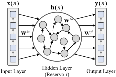
Despite efficient fitting of sequential data via ESN, some limitations worth considering: 1) ESN only captures the datainherent dynamics within the fitting direction (often the datacollection order), while dynamics in other directions are not considered; 2) The size of the fitted ESN model increases linearly with the size of the input/output value, resulting in redundant fitted models when fitting multi-dimensional data, a non-conducive situation for further processing on the models.
3 Methodology
This section details our approach: 1) Each data instance is fitted with REDNet to capture its multi-directional dynamics and is then represented by an individual fitted REDNet model; 2) We adopt a practical distance metric to assess the differences between fitted models; 3) Representing instances with fitted models, supported with the distance metric between models, FD is implemented in REDNet model space.
3.1 Reservoir-Embedded-Directional Network
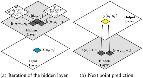
Similar to ESN (Figure 2), REDNet consists of an input layer, a hidden layer, and an output layer. But unlike ESN, the hidden layer of REDNet is made of K reservoirs with M units each, aiming to capture dynamics in K directions. Each reservoir consists of interconnected neurons, linked by fixed and randomly established connections. Figure 3 shows the REDNet structure for capturing dynamics in 2 directions.
Suppose a K-directional correlated data instance 2 , a point is positioned by (n1, n2, ..., nK), where ni ∈ [1,Ni] indicates the coordinate along the ith direction. The input value, hidden state, and output value at point (n1, n2, ..., nK) are represented by x(n1, n2, ..., nK), h(n1, n2, ..., nK) and y(n1, n2, ..., nK), respectively. The iteration formula of REDNet is defined as:
2 In this paper, "K-directional correlated" means that there are correlations within K directions in the data. "K-directional correlated data" could be abbreviated as "K-directional data".
whereWhh = [Whh1 ,Whh2 , ...,WhhK ] indicate the fixed, randomly determined reservoir weights that describe neuron connections in the reservoir, fulfilling the Echo State Property [Jaeger, 2001] with a spectral radius between 0 and 1; Whx refer to the input weight, randomly assigned fixed values from -1 to 1; g is the activation function tanh. The initial hidden state h(0, n2 · · · , nK) = h(n1, 0, · · · , nK) = · · · = h(n1, n2, · · · , 0) = 0 in each direction.
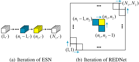
The hidden-state iteration of REDNet is started from point (1, 1, ..., 1) to point (N1,N2, ...,NK), with the process exampled in Figure 4. Each point is correlated with surrounding processed points. Specifically, according to Equation (3), the hidden state of a point is influenced not only by the input value of the current point, but also by the hidden states of the surrounding processed points within different directions. This effect persists as the iteration progresses, thereby establishing a network of connections between each point in the data and previously processed points in different directions.
After computing the hidden states for all points, as illustrated in Figure 3(b), the output layer calculates the output value y for each point based on the previous hidden states:
whereWyh = [Wyh1 ,Wyh2 , ...,WyhK ] refer to the output weights of REDNet, and a indicates the bias.
The fitting process is accomplished by a prediction task on the original instance, that is, approximating y(n1, ..., nK) to x(n1, ..., nK) to build the connection between the current input value and the hidden states of processed points. Thus, the output weight Wyh and bias a could be directly estimated via regression [Chen et al., 2024]. Through the above fitting, the correlation between adjacent data points is modeled by REDNet's multi-reservoir architecture and unique iterative approach. The multi-directional dynamics within the data are captured and encoded into a compact REDNet model, represented in the function form as:
where h = [h(n1 - 1, ..., nK); ...; h(n1, ..., nK - 1)] represents the concatenated hidden states of the processed points, Wyh = [Wyh1 , · · · ,WyhK ] refer to the output weights, and a is the bias vector. Figure 3 illustrates the iteration and prediction of REDNet when handling 2-directional data.
In terms of model size and memory usage, when handling K-directional data, REDNet provides the output weight of size K ×M, where M refers to the number of units in each reservoir within the hidden layer. In comparison, suppose ESN is employed to fit the data along the jth direction, the
size of its output weight is K∏ i=1,i̸=j Ni ×M, where Ni repre-
sents the number of values in the ith direction.
For example, consider a typical 2-directional data instance of 100 dimensions (synchronous measurements) and 1000 time points (data-collection order), represented as size 100 × 1000, where efficient changing information exists both in the data-collection order and among synchronous measurements. Using the prediction formula in Equation (4), REDNet's output weight is 2×M, where M represents the number of units per reservoir in the hidden layer. In contrast, using ESN to fit data along the data-collection order results in an output weight of 100 × M. Therefore, REDNet provides a more compact model with significantly reduced memory requirements. Additionally, REDNet achieves data fitting solely through ridge regression, eliminating the need for iterative offline training or optimization and ensuring manageable computation in time-sensitive tasks.
3.2 Distance Metric betweenModels
Following the data fitting through REDNet, the distance between the fitted models is defined to measure the difference between models. Supposing two K-directional data instances are fitted by REDNet, the two models could be represented by:
The 2-norm distance [Chen et al., 2013b] between models f1(h) and f2(h) is adopted in this paper, estimated by:
where Wyh 12 =Wyh 1 -Wyh 2 , a12 = a1-a2. aT12 is the transpose of a12. f1 and f2 are the simplified representations of models f1(h) and f2(h). Since tanh serves as the activation function g in Equation (3), h ∈ [-1, 1]KM and the integral range C ∈ [-1, 1]KM .
Note that for any fixed a12 andWyh 12 , there is
in the integral range C ∈ [-1, 1]KM , since the integrand is an odd function. Therefore:
where wj is the (1, j)th element ofWyh 12 .
We then scale of the squared model distance L22 (f1, f2) by 2-KM , and obtain:
Via Equation (10), the distance between two models is directly measured, enabling the utilization of distance-based learning algorithms on these models.
3.3 Fault Diagnosis in REDNet Model Space
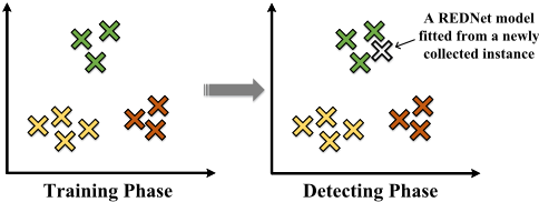
Fault Diagnosis (FD) involves classifying unknown data instances as either normal or specific fault types. As illustrated in Figure 5, our approach consists of two phases, i.e., the "Training phase" and "Detection phase".
Training Phase
Each labeled data instance is fitted using REDNet, obtaining a corresponding fitted model. This fitted model represents the original data instance, mapping it into the REDNet model space. A classifier, such as Support Vector Machine (SVM) [Cortes and Vapnik, 1995] or K-Nearest Neighbors (KNN) [Altman, 1992], is then trained on these models, supported by the distance metric between models.
Detection Phase
Given a newly collected data instance, it is fitted with REDNet. The fitted model is then evaluated using the previously trained classifier to determine whether it is normal or belongs to a specific fault type, directly corresponding to the type of the original data instance.
4 Experimental Study
The experiments are conducted with an Intel Xeon E5-2650 v3 CPU and NVIDIA GeForce RTX 3090 GPU, running MATLAB R2021a and Python 3.8. The default settings of REDNet include a spectral radius of 0.7 and a reservoir size of 60. In the REDNet model space, SVM is adopted 3 by default for classification, and other classifiers are subsequently evaluated.
4.1 The Utilzied Datasets
The experiments employ four well-known FD datasets, including CWRU 4 , SMD 5 , TBV 6 and GFD 7 . Specifically, to address scenarios with limited labeled data, we constrain the training data to just 50 samples per category across all utilized datasets, with the remaining serving for testing.
- Gearbox Fault Diagnosis Dataset (GFD) [Ghanbari et al., 2023] consists of 4-dimensional vibration signals collected by SpectraQuest's Gearbox Fault Diagnostics Simulator under varying load conditions. It supports binary classification (healthy and broken tooth) with data
3 Implementation from scikit-learn: https://scikit-learn.org.
4 https://engineering.case.edu/bearingdatacenter
5 https://github.com/NetManAIOps/OmniAnomaly
6 https://data.mendeley.com/datasets/fm6xzxnf36/2
7 https://www.kaggle.com/datasets/brjapon/ gearbox-fault-diagnosis
| Method | GFD | TBV SMD | CWRU-A CWRU-B | CWRU-E | ||||||
|---|---|---|---|---|---|---|---|---|---|---|
| Pre | Rec F1 | Pre Rec F1 Pre Rec | F1 Pre Rec | F1 | Pre Rec F1 | CWRU-C Pre Rec F1 | CWRU-D Pre Rec F1 | Pre Rec F1 | ||
| GRU | 99.3 99.0 | 99.2 | 73.0 72.9 72.9 | 96.7 96.4 96.5 | 87.9 87.5 87.7 | 95.1 | 95.0 95.0 83.8 83.8 | 83.6 97.6 97.8 97.7 | 98.7 98.7 98.7 | |
| DTL-CWT | 98.3 98.2 98.2 | 63.8 | 60.3 62.0 95.8 95.7 | 95.7 97.6 97.6 | 97.6 | 98.6 98.7 98.6 | 98.8 98.7 98.7 | 98.6 98.7 98.6 | 97.1 97.0 97.0 | |
| TimesNet | 94.0 94.1 94.1 | 58.1 50.3 53.9 | 95.6 97.5 96.5 | 73.4 71.6 | 72.5 | 74.5 63.3 68.4 | 78.6 74.5 70.9 | 86.1 79.3 80.4 | 87.1 85.5 85.0 | |
| Convnext-V2 | 91.5 91.2 91.4 | 79.6 79.5 79.5 | 99.3 99.3 99.3 | 98.6 98.6 | 98.6 | 98.1 98.6 98.3 | 99.2 99.0 99.1 | 98.3 98.5 99.4 | 98.5 99.1 98.8 | |
| Swin-Trans | 98.6 98.4 98.5 | 96.0 95.5 95.7 | 96.6 96.4 96.5 | 97.2 97.7 97.4 | 98.9 98.9 98.9 | 99.4 99.5 99.4 | 98.8 98.3 98.6 | 98.8 98.8 98.8 | ||
| FEDformer | 92.5 92.3 92.3 | 60.2 59.6 59.9 | 92.6 92.2 92.4 | 58.8 58.0 | 58.4 | 54.2 55.3 54.7 | 54.0 54.9 54.4 | 62.1 59.7 60.9 | 76.2 75.6 75.9 | |
| Autoformer | 94.1 94.0 94.0 | 54.0 49.3 51.6 | 93.8 93.6 93.6 | 64.5 58.0 | 61.1 | 65.9 65.5 65.4 | 61.7 60.3 61.0 | 74.2 72.6 73.4 | 84.6 84.1 84.3 | |
| ESN-MS | 95.1 94.7 95.9 | 89.0 91.3 90.1 | 92.8 93.6 93.2 | 95.2 95.0 95.1 | 95.5 95.3 95.4 | 97.1 96.3 96.7 | 95.6 93.3 94.4 | 94.9 94.6 94.7 | ||
| REDNet (E/d) | 96.2 96.0 96.1 | 90.8 92.8 91.6 | 95.3 95.2 95.2 | 96.7 96.5 | 96.6 96.8 | 96.6 96.7 | 98.5 97.6 | 98.0 96.9 94.5 95.6 | 96.2 95.8 | 96.0 |
| Our Approach | 99.1 98.9 99.0 | 99.3 98.8 99.0 | 99.8 99.7 99.7 | 98.9 99.2 99.0 | 99.1 | 99.1 99.1 | 99.7 99.7 | 99.7 98.9 98.8 98.9 | 99.3 99.4 | 99.3 |
instances of length 1024, comprising 100 instances for each load condition.
- Triaxial Bearing Vibration Dataset (TBV) [Kumar et al., 2022] contains 3-dimensional vibration data collected from an induction motor's bearing housing under varying conditions. It supports a 13-class classification task, including one healthy and 12 faulty states (inner and outer race defects with six severity levels each). The dataset consists of instances of length 1024, with 100 instances extracted for each condition.
- Server Machine Dataset (SMD) [Su et al., 2019] contains 38-dimensional sequential data collected from 28 machines over five weeks. It supports binary classification, distinguishing between normal and anomalous states, with instances of length 256. For this study, 1000 instances were extracted from both normal and anomalous scenarios for analysis.
- Case Western Reserve University Bearing Dataset (CWRU) [Loparo, 2012] comprises vibration signals from bearings in 2 dimensions, recorded under four different load conditions (sub-datasets A, B, C, and D). These datasets include 10 classes: one normal class and nine distinct anomaly classes. Each sub-dataset contains 200 instances per category, with a length of 1024. Additionally, the combination of A-D is denoted as E.
System operations introduce correlations in the "time direction", that is, the order of data collection. Additionally, synchronous measurements from multiple sensors exhibit systematic correlations. Therefore, it is essential to capture the dynamics both in the "time" and "sensor" directions (K = 2) to ensure comprehensive data analysis.
4.2 Baseline Methods
We evaluate our approach against recent baselines, including: 1) RNN-based methods process temporal data point by point, i.e., the Gated Recurrent Units (GRU) [Cho et al., 2014]; 2) Image-format-based methods that convert time series signals into image-shaped data through wavelet transformation, including Deep Transfer Learning with Continuous Wavelet Transform (DTL-CWT) [Shao et al., 2019], Convnext-V2 (base model) [Woo et al., 2023], and Swin Transformer (Swin-Trans) [Liu et al., 2021]; 3)
Transformer-based methods utilize self-attention mechanisms to handle dependencies in data sequences, including FEDformer [Zhou et al., 2022], Autoformer [Wu et al., 2021] and TimesNet [Wu et al., 2023].
4.3 Results and Discussion
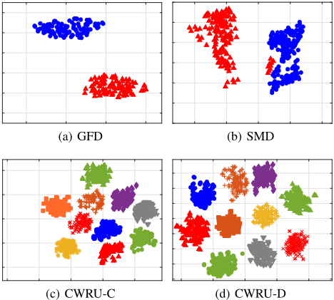
The results 8 are shown in Table 1. Our method consistently delivers substantial results across all datasets. REDNet effectively captures and represents the distinct dynamics induced by fault occurrences, both within the data collection direction and across synchronous measurements. Consequently, models derived from fault conditions significantly differ from those of normal data and other fault types, as evident in Figure 6. While DTL-CWT and Swin-Trans perform well on the GFD and CWRU datasets, they struggle with more complex dynamics. Our approach, focusing on intrinsic dynamics, requires minimal training data. With only 50 samples per class, DL methods, particularly those reliant on extensive neural networks, struggle to converge rapidly and efficiently. Future experiments will further investigate FD effectiveness with limited data and compare training durations.
8 All evaluated methods show a standard deviation of less than 2% across more than five repetitions, indicating stable outcomes. ESN-MS and REDNet(E/d) are discussed in the Ablation Study.
Discussion with Limited Training Data
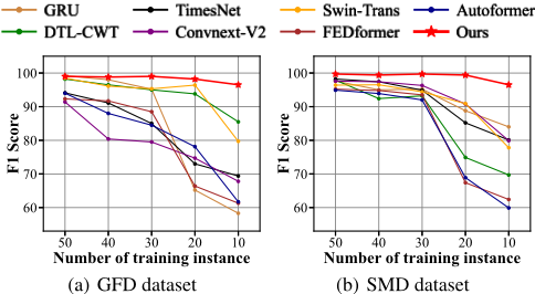
We selected the GFD and SMD datasets where all baselines initially excelled. Figure 7 shows the F1-Scores of our method and others as training data decreases from 50 to 10 instances per category. Our approach, leveraging inherent data dynamics, represents data with dynamic-captured fitted models for classification. Figure 6 demonstrates that consistent conditions produce similar REDNet models, while different fault types lead to significant disparities due to varied dynamics captured. Remarkably, our method maintains F1scores above 90% even when training data is limited to just 10 instances per class. Conversely, the performance of traditional DL methods, including those using pre-trained models for transfer learning, deteriorates sharply with reduced data.
Training Times of Evaluated Methods
Rapid training post-data acquisition is essential for practical FD tasks 9 . Table 2 details the training times for various methods. DL approaches, including those using transfer learning, typically require extended periods for convergence. Imagebased methods, such as Swin-Transformer, incur additional delays due to the conversion of time-series data into spectrograms. In contrast, REDNet employs straightforward ridge regression for efficient data fitting, bypassing iterative optimization, and utilizes established distance-based classifiers like SVM for swift model classification.
Ablation Study
Our approach features: 1) Multiple reservoirs in REDNet's hidden layer to adequate dynamic capture; and 2) A directsolvable model distance measurement to evaluate the difference between REDNet models.
9 All methods achieve inference within 0.1 seconds per instance, satisfying the time requirements of most FD tasks, thus the inference time is not discussed here.
| CWRU | ||||||||
|---|---|---|---|---|---|---|---|---|
| Method | GFD | TBV | SMD | A | B | C | D | E |
| GRU | 104.9 | 565.93 | 11.4 | 434.4 | 445.9 | 440.6 | 429.2 | 1771.0 |
| DTL-CWT | 246.4 | 435.5 | 78.7 | 98.5 | 99.5 | 98.8 | 98.5 | 349.0 |
| Convnext-V2 | 52.5 | 316.6 | 53.1 | 244.6 | 243.9 | 243.0 | 245.0 | 978.3 |
| Swin-Trans | 193.7 | 578.2 | 224.5 | 449.6 | 450.6 | 449.1 | 447.8 | 1777.2 |
| TimesNet | 116.8 | 417.1 | 65.6 | 321.5 | 331.8 | 358.9 | 366.7 | 420.4 |
| Autoformer | 49.4 | 227.0 | 29.5 | 113.3 | 121.8 | 122.4 | 114.5 | 177.5 |
| FEDformer | 224.7 | 921.8 | 139.3 | 580.8 | 559.0 | 565.5 | 568.9 | 2177.0 |
| Our Approach | 1.2 | 13.6 | 2.1 | 9.8 | 8.4 | 8.6 | 8.2 | 12.5 |
| KNN | Random Forest | |||||
|---|---|---|---|---|---|---|
| Classifier | Pre | Rec | F1 | Pre | Rec | F1 |
| GFD | 97.5% | 98.1% | 97.8% | 97.1% | 97.5% | 97.3% |
| TBV | 98.1% | 98.5% | 98.3% | 98.1% | 98.1% | 98.1% |
| SMD | 99.2% | 99.6% | 99.4% | 98.5% | 98.8% | 98.6% |
| CWRU-Avg | 98.6% | 98.9% | 98.9% | 98.4% | 98.7% | 98.4% |
Instead of multi-directional dynamic capture, we use ESN for single-directional fitting and classifying the fitted ESN model, denoted as ESN-model-space (ESN-MS). Also, we replaced our model distance metric with original Euclidean distance in the subsequent FD process, denoted by REDNet (E/d). Table 1 indicates that capturing multi-directional dynamics is proven to be 5% more effective than relying on single-directional fitting (ESN-MS). Compared with REDNet (E/d), using our proposed model distance metric can also improve the classification effect by about 3%, as it more reasonably measures the differences between models, with varying contributions from output weights and bias.
Different Classifiers in the REDNet Model Space
The performance of KNN and Random Forest (RF) within the REDNet model space is shown in Table 3, using default experimental settings. According to Table 1, SVM outperforms, with KNN also yielding better results than RF. As depicted in Figure 6, models from similar data types cluster closely, enhancing category discrimination. Consequently, these three methods outperform other baseline approaches in Table 1.
5 Conclusion
This paper introduces FD within the REDNet model space, validated across various datasets. REDNet captures multidirectional dynamics, mapping data into a class-separable model space. Our approach independently fits each instance using ridge regression, significantly reducing training time. Focusing on data-intrinsic dynamics enables FD with minimal training data. Future work will explore REDNet's impact on more directional correlated data. For data with more directional correlations, how to adaptively adjust the strength of correlations in different directions is also worthy of study.
Acknowledgments
This work was supported in part by the National Natural Science Foundation of China (No. 62206261, 62137002, 62176245), in part by the Fundamental Research Funds for the Central Universities (No. WK2150110039).
@inproceedings{ijcai2025p802,
  title     = {Fault Diagnosis in REDNet Model Space},
  author    = {Zhou, Xiren and Tang, Ziyu and Liu, Shikang and Chen, Ao and Wang, Xiangyu and Chen, Huanhuan},
  booktitle = {Proceedings of the Thirty-Fourth International Joint Conference on
               Artificial Intelligence, {IJCAI-25}},
  publisher = {International Joint Conferences on Artificial Intelligence Organization},
  editor    = {James Kwok},
  pages     = {7209--7217},
  year      = {2025},
  month     = {8},
  note      = {Main Track},
  doi       = {10.24963/ijcai.2025/802},
  url       = {https://doi.org/10.24963/ijcai.2025/802},
}
TY - CPAPER TI - Fault Diagnosis in REDNet Model Space AU - Zhou, Xiren AU - Tang, Ziyu AU - Liu, Shikang AU - Chen, Ao AU - Wang, Xiangyu AU - Chen, Huanhuan T2 - Proceedings of the Thirty-Fourth International Joint Conference on Artificial Intelligence, IJCAI-25 PB - International Joint Conferences on Artificial Intelligence Organization PY - 2025 SP - 7209 EP - 7217 DO - 10.24963/ijcai.2025/802 UR - https://doi.org/10.24963/ijcai.2025/802 ER -Copied
Machine-readable versions of this paper, for tools and AI agents:





