
Dynamic Replanning for Improved Public Transport Routing
Proceedings of the Thirty-Fourth International Joint Conference on Artificial Intelligence. Main Track. Pages 8430-8437.
https://doi.org/10.24963/ijcai.2025/937
Keywords
- Planning and Scheduling: PS: Planning under uncertainty
- Planning and Scheduling: PS: Routing
- Planning and Scheduling: PS: Real-time planning
- Planning and Scheduling: PS: Search in planning and scheduling
Abstract
Delays in public transport are common, often impacting users through prolonged travel times and missed transfers. Existing solutions for handling delays remain limited; backup plans based on historical data miss opportunities for earlier arrivals, while snapshot planning accounts for current delays but not future ones. With the growing availability of live delay data, users can adjust their journeys in real-time. However, the literature lacks a framework that fully exploits this advantage for system-scale dynamic replanning. To address this, we formalise the dynamic replanning problem in public transport routing and propose two solutions: a "pull" approach, where users manually request replanning, and a novel "push" approach, where the server proactively monitors and adjusts journeys. Our experiments show that the push approach outperforms the pull approach, achieving significant speedups. The results also reveal substantial arrival time savings enabled by dynamic replanning.
- [Abuaisha et al., 2024] Abdallah Abuaisha, Mark Wallace, Daniel Harabor, and Bojie Shen. Efficient and exact pub- lic transport routing via a transfer connection database. In Proceedings of the International Symposium on Combina- torial Search, volume 17, pages 2-10, 2024.
- [Bast et al., 2010] Hannah Bast, Erik Carlsson, Arno Eigen- willig, Robert Geisberger, Chris Harrelson, Veselin Ray- chev, and Fabien Viger. Fast routing in very large pub- lic transportation networks using transfer patterns. In Algorithms-ESA 2010: 18th Annual European Sympo- sium, Liverpool, UK, September 6-8, 2010. Proceedings, Part I 18, pages 290-301. Springer, 2010.
- [Bast et al., 2013] Hannah Bast, Jonas Sternisko, and Sabine Storandt. Delay-robustness of transfer patterns in public transportation route planning. In ATMOS-13th Workshop on Algorithmic Approaches for Transportation Modelling, Optimization, and Systems-2013, volume 33, pages 42- 54. Schloss Dagstuhl-Leibniz-Zentrum fuer Informatik, 2013.
- [Baum et al., 2023] Moritz Baum, Valentin Buchhold, Jonas Sauer, Dorothea Wagner, and Tobias Zündorf. Ultra: Un- limited transfers for efficient multimodal journey plan- ning. Transportation Science, 57(6):1536-1559, 2023.
- [Botea et al., 2013] Adi Botea, Evdokia Nikolova, and Michele Berlingerio. Multi-modal journey planning in the presence of uncertainty. In Proceedings of the Interna- tional Conference on Automated Planning and Scheduling, volume 23, pages 20-28, 2013.
- [Cionini et al., 2017] Alessio Cionini, Gianlorenzo D'Angelo, Mattia D'Emidio, Daniele Frigioni, Kalliopi Giannakopoulou, Andreas Paraskevopoulos, and Christos Zaroliagis. Engineering graph-based models for dynamic timetable information systems. Journal of Discrete Algorithms, 46:40-58, 2017.
- [Delling et al., 2015a] Daniel Delling, Julian Dibbelt, Thomas Pajor, and Renato F Werneck. Public transit labeling. In Experimental Algorithms: 14th International Symposium, SEA 2015, Paris, France, June 29-July 1, 2015, Proceedings 14, pages 273-285. Springer, 2015.
- [Delling et al., 2015b] Daniel Delling, Thomas Pajor, and Renato F Werneck. Round-based public transit routing. Transportation Science, 49(3):591-604, 2015.
- [Dibbelt et al., 2014] Julian Dibbelt, Ben Strasser, and Dorothea Wagner. Delay-robust journeys in timetable networks with minimum expected arrival time. In 14th Workshop on Algorithmic Approaches for Transportation Modelling, Optimization, and Systems (2014). Schloss- Dagstuhl-Leibniz Zentrum für Informatik, 2014. [Dibbelt et al., 2018] Julian Dibbelt, Thomas Pajor, Ben Strasser, and Dorothea Wagner. Connection scan algo- rithm. Journal of Experimental Algorithmics (JEA), 23:1- 56, 2018.
- [Dijkstra, 1959] Edsger W. Dijkstra. A note on two prob- lems in connexion with graphs. Numerische Mathematik, 1:269-271, 1959.
- [D'Emidio and Khan, 2019] Mattia D'Emidio and Imran Khan. Dynamic public transit labeling. In International Conference on Computational Science and Its Applica- tions, pages 103-117. Springer, 2019.
- [Hansen, 2001] Ingo A Hansen. Improving railway punc- tuality by automatic piloting. In ITSC 2001. 2001 IEEE Intelligent Transportation Systems. Proceedings (Cat. No. 01TH8585), pages 792-797. IEEE, 2001.
- [Marković et al., 2015] Nikola Marković, Sanjin Milinković, Konstantin S Tikhonov, and Paul Schon- feld. Analyzing passenger train arrival delays with support vector regression. Transportation Research Part C: Emerging Technologies, 56:251-262, 2015.
- [Phan and Viennot, 2019] Duc-Minh Phan and Laurent Vi- ennot. Fast public transit routing with unrestricted walking through hub labeling. In International Symposium on Ex- perimental Algorithms, pages 237-247. Springer, 2019.
- [Redmond et al., 2022] Michael Redmond, Ann Melissa Campbell, and Jan Fabian Ehmke. Reliability in public transit networks considering backup itineraries. European Journal of Operational Research, 300(3):852-864, 2022.
- [Simmons, 1992] Reid G Simmons. Concurrent planning and execution for autonomous robots. IEEE Control Sys- tems Magazine, 12(1):46-50, 1992.
- [Zhang et al., 2024] Yue Zhang, Zhe Chen, Daniel Harabor, Pierre Le Bodic, and Peter J. Stuckey. Planning and execu- tion in multi-agent path finding: Models and algorithms. In Proceedings of the Thirty-Fourth International Con- ference on Automated Planning and Scheduling, ICAPS 2024, Banff, Alberta, Canada, June 1-6, 2024, pages 707- 715. AAAI Press, 2024.
References were extracted automatically from the PDF and may contain errors.
Full text extracted automatically from the PDF; figures, tables and equations may differ. The PDF is the version of record.
1 Introduction
Public transport is a crucial component of smoothly functioning urban mobility systems. Unfortunately, in dynamic environments, travel conditions can change rapidly and unexpected incidents can occur, making delays in public transport fairly common. These delays often result in missed transfers, prolonged travel times, and late arrivals for users. Efficient routing that accounts for real-time delays can play a vital role in reducing travel times for users, ultimately enhancing their satisfaction and trust in the public transport system.
To handle dynamic scenarios, many works utilise historical delay data or delay probability distributions. Backup plans (i.e., a policy) are precomputed offline, with the objective of maximising reliability by providing plans that remain viable when potential delays occur, or minimising expected arrival time at the destination [Botea et al., 2013; Dibbelt et al., 2014; Redmond et al., 2022]. These plans, which can be printed in advance, offer multiple options at each transfer stop for users to consult in case of disruptions. However, these contingent planning approaches fail to account for all possible scenarios and only address delays of limited duration, potentially missing opportunities for earlier arrivals. Another family of algorithms demonstrates the feasibility of efficiently updating timetables [Cionini et al., 2017; Dibbelt et al., 2018] or precomputed data structures [D'Emidio and Khan, 2019; Baum et al., 2023] to account for delays. While this can enable snapshot planning with updated information, resulting journeys may be infeasible or suboptimal due to unforeseen future delays.
With widespread internet access, many transport operators and journey-planning applications, such as Google Maps, provide real-time data, including service disruptions and updated vehicle departure and arrival times. This enables users to manually review updates and request replanning when necessary. Dynamic replanning, a widely adopted concept, enables real-time adaptation to environmental changes, addressing the limitations of offline and snapshot planning. By leveraging updated information and computational techniques, it enhances efficiency and reliability in applications such as robotics [Simmons, 1992] and multi-agent systems [Zhang et al., 2024]. However, extending dynamic replanning to public transport routing is challenging. The number of replans and the search space required for a single journey often exceed expectations. Not only disruptions directly impacting the journey (e.g., a missed transfer or a delayed service) must be considered, but also those affecting other services in the network, which can sometimes lead to an earlier arrival time at the destination. Consequently, frequent replanning is essential, with each replan accounting for all timetable services.
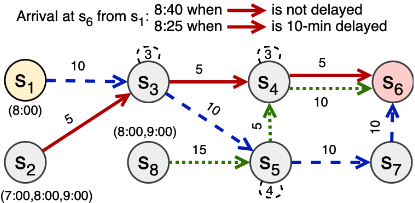
Example 1. Consider Figure 1. Departing from the origin stop s1 at 8:00, the original optimal plan, according to the normal timetable, involves taking the 8:00 trip on route r1, t1, and arriving at the destination stop s6 at 8:40. However, if the 8:00 trip on route r2, t2, is delayed by 10 minutes while t1 runs on schedule, then catching the delayed t2 at stop s3 becomes possible. The updated optimal plan involves taking t1 from s1, then changing at s3 to t2, which arrives at s6 at 8:25, earlier than the original plan's arrival time of 8:40.
To the best of our knowledge, we are the first to extend the dynamic replanning concept to public transport routing. We begin by providing a comprehensive description and formulation of the problem. Next, we propose a straightforward pull approach, where users frequently request real-time journey replans from a central server via their edge devices (e.g., mobile phones), utilising the typical centralised setup for managing queries. However, the pull approach has several drawbacks: (i) it is inconvenient for users due to frequent manual actions, such as monitoring updates and requesting replans; (ii) it relies on user judgement, which may lead to missed opportunities for earlier arrivals; and (iii) it places pressure on the server with numerous requests, reducing efficiency and complicating timetable updates. To address these issues, we further propose a novel push approach, where the server continually monitors and adjusts user journeys, pushing revised plans to users' edge devices. While more convenient for users, simply replanning strains the server, as it must monitor and replan for all users based on the entire timetable. To improve efficiency, the server creates a query-specific envelope, containing only relevant timetable parts. This envelope is sent to the edge device, which subscribes to envelope updates and performs local replanning on the envelope, reducing the search space and distributing the computational load.
Our extensive experiments on metropolitan datasets reveal two key findings: (i) the push approach achieves significant query efficiency, delivering runtimes within a fraction of a second, an order of magnitude faster than the pull approach, while enabling the capacity to process 10-20 times more queries; and (ii) our dynamic replanning strategy saves 5-30 minutes per journey on average compared to static and other dynamic strategies, even when the initial plan is not delayed.
2 Preliminaries
2.1 Timetable Modelling
The timetable is the main input for any public transport routing system. We follow one of the most popular methods, as detailed in Dibbelt et al. (2018), which directly utilises the timetable structure rather than constructing a graph. Specifically, we represent a timetable as TB = (S, T, C, F), where S denotes stops, T denotes trips, C denotes connections, and F denotes footpaths. Each component is defined as follows:
- A stop s ∈ S is a departure and/or arrival point where a vehicle stops to pick up and/or drop off passengers.
- A trip t ∈ T corresponds to a scheduled transport vehicle that visits a specific order of stops. Trips with the same order of stops can be grouped into a route.
- Each trip t ∈ T is divided into a sequence of connections,
denoted as tC = ⟨c0, c1, . . . , ck⟩. A connection c ∈ tC is represented as a 5-tuple (sdep, τdep, sarr, τarr, t), indicating an event where trip t departs from stop sdep ∈ S at time τdep and arrives at stop sarr ∈ S at time τarr, with no intermediate stops. Note that sdep ̸= sarr and τdep < τarr always hold. Connections in tC satisfy the following properties: 1 (i) t(c0) = t(c1) = · · · = t(ck), (ii) sdep(ci) = sarr(ci-1), and (iii) τdep(ci) ≥ τarr(ci-1), ∀i ∈ {1 . . . k}. The union of all connections from all trips in T forms the full set C.
· A footpath f ∈ F models walking between two stops to change trips. It is represented as a triple f = (si, sj,∆τ(si, sj)), indicating a transfer from stop si ∈ S to stop sj ∈ S with a duration of ∆τ(si, sj). We require each stop si ∈ S to have a loop footpath f = (si, si,∆τ(si, si)). Each stop si ∈ S is associated with a list of its outgoing footpaths, denoted as f(si) = {f0, . . . , fm} ⊆ F. Following Dibbelt et al. (2018), footpaths are required to satisfy the transitive closure and triangle inequality properties.
A journey in TB is a scheduled path from origin stop so to destination stop sd. It consists of a sequence of connections j = ⟨c0, . . . , cn⟩, where sdep(c0) = so and sarr(cn) = sd. Each pair of consecutive connections either shares the same trip t ∈ T (i.e., no vehicle change) or requires a transfer via a footpath f ∈ F. Each transfer must respect the required transfer time. Formally, τarr(ci-1) +∆τ(sarr(ci-1), sdep(ci)) ≤ τdep(ci) must hold ∀i ∈ {1 . . . n}.
Earliest Arrival Time Problem (EATP). Given a query q = (so, sd, τq), EATP aims to find a journey j that departs from origin so no earlier than time τq and arrives at destination sd as early as possible, at time τd, assuming no delays in timetable TB. Such a journey is denoted as j(so, sd, τq).
2.2 DelayModelling
The dynamic nature of public transport networks often causes disruptions, such as traffic congestion, technical issues, and adverse weather, leading to service delays. These delays can significantly affect travel plans computed based on published timetables, resulting in missed transfers and longer travel times. To model delays, we assume the transport system operates a centralised server that stores the original timetable TB and also maintains a list of delay events DV .
Definition 1. (Delay Event). A delay event dv ∈ DV is represented as a tuple (t, τδ, δ), where t ∈ T denotes the trip experiencing the delay, τδ specifies the time when the delay occurs, and δ represents the duration of the delay. The time τδ must fall within the trip's timeframe (i.e., τdep(c0) ≤ τδ ≤ τarr(ck) for t = ⟨c0, . . . , ck⟩).
When a delay event occurs, it impacts all subsequent connections in trip t after time τδ. To avoid synchronisation issues, we assume the real-time timetable TBcurr at time τcurr can be derived from the original timetable TB and the delay events DV . This requires identifying each delayed trip t based on DV , scanning its affected connections c in TB, and adjusting their departure and arrival times according to the trip's delay δ (i.e., τdep(c) = τdep(c) + δ and
1 We often use the notation a(b) to denote "a of b", unless stated otherwise. For instance, t(ci) refers to the trip of connection ci.
τarr(c) = τarr(c) + δ). Unlike previous works, we do not impose any restrictions on the maximum duration of delays.
Snapshot Earliest Arrival Time Problem (SEATP). Given a query q = (so, sd, τq, DV ), SEATP plans a journey j as in EATP, but while accounting for current delay events DV in a snapshot of timetable TB, denoted as TBcurr .
2.3 Snapshot Solver
Several EATP algorithms can be adapted to solve SEATP, with the Connection Scan Algorithm (CSA) [Dibbelt et al., 2018] being one of the most efficient online approaches. Below, we provide a brief overview of CSA.
Unlike Dijkstra's algorithm [Dijkstra, 1959], CSA does not operate on a graph and does not require a priority queue. Instead, it compiles all connections from a timetable TB into a single array C, sorted by (updated) departure time (i.e., from earliest to latest), and efficiently solves queries by scanning through this sorted array. Specifically, CSA maintains an array A to store the tentative earliest arrival time for each stop s ∈ S. Initially, A is set to infinity for all stops. Next, A at each stop si that is walking-reachable from the origin stop so via a footpath in f(so) is updated to τq +∆τ(so, si). The algorithm then proceeds to scan the connections in C in sequential order, starting from the first connection that departs at or after τq. For each scanned connection c, the algorithm first checks its reachability. A connection is considered reachable if there exists a way to catch it on time (e.g., A[sdep(c)] ≤ τdep(c)). If c is reachable and can improve the arrival time at sarr(c), the algorithm updates A at each accessible stop sj via an outgoing footpath from sarr(c), if A[sj] can be improved. Since sarr(c) has a loop transfer, its own arrival time, A[sarr(c)], is also updated. However, if c is not reachable, the algorithm simply skips it and proceeds to the next connection. This process continues until all connections in C departing before A[sd] are scanned. Finally, the algorithm returns the arrival time at the destination stop, A[sd]. To extract the full journey, the algorithm is augmented with journey pointers or followed by a post-processing phase. For further details, refer to Dibbelt et al. (2018).
3 Dynamic Replanning
Both contingent and snapshot planning may miss opportunities to improve arrival times. Building on its success in various domains, we propose a dynamic replanning approach to address this limitation. Dynamic replanning involves adapting and improving plans during execution to effectively handle uncertainties in constantly changing real-time environments. The core of our approach is to initially provide passengers with an optimal plan, which is then proactively and continually adjusted as necessary along their journey based on the latest delay information. The goal is to reduce the impact of disruptions on passenger travel times. A key observation is that passengers cannot take any action while the vehicle is in motion between stops. Therefore, replanning just before arriving at each stop along the journey until reaching the destination is sufficient, providing the finest feasible time granularity. In broad terms, our dynamic replanning strategy for solving a single user query consists of the following steps:
- Update the original timetable TB with the latest delay events DV at the current time τcurr to derive the real-time timetable TBcurr .
- Plan an optimal snapshot journey j from the current stop scurr to the destination stop sd using the current timetable TBcurr with an SEATP solver.
- Execute the first action of the planned journey j, which depends on the current travel context.
Steps 1 to 3 are repeated iteratively at each stop, starting from the origin so as the current stop scurr, until the passenger reaches the destination sd. Let c be the first connection of the newly planned journey j in the current iteration, and c′ the connection taken in the previous iteration. The action the passenger should execute at the end of the current iteration falls into one of four cases 2 : (i) catch the trip with connection c directly from s0, if c′ is null; (ii) stay on the current trip, if c and c′ belong to the same trip; (iii) alight from the current trip at stop sarr(c′ ) and board a new trip at stop sdep(c), if c and c′ belong to different trips; or (iv) reach sd directly by walking via a footpath, if c is null. Cases (i), (ii), and (iv) are straightforward. In case (iii), we consider walking from sarr(c′ ) to sdep(c) and boarding connection c as a single action, without any intermediate replanning, assuming the user is committed to this course of action.
Regarding the snapshot solver, offline preprocessing-based algorithms are generally unsuitable for frequent replanning due to the high cost of repairing precomputed data [Bast et al., 2010; Delling et al., 2015a; Baum et al., 2023; Abuaisha et al., 2024]. In contrast, online algorithms such as CSA [Dibbelt et al., 2018] and RAPTOR [Delling et al., 2015b] are better suited, as they support timetable updates at a relatively low computational cost. In this paper, we adopt CSA as the underlying replanning solver; however, any solver designed for a similar timetable structure could also be used.
4 Our Approaches
We introduce two approaches for dynamic replanning: a baseline pull approach and a more efficient push approach.
4.1 The Pull Approach
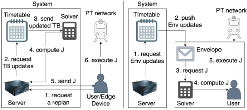
The straightforward approach follows the conventional setup where a central server handles all user queries in the network. In this approach, users frequently request (pull) journey replans from the server via their edge devices. We assume users recognise the need to replan at every stop along their journey, in line with our formulation of dynamic replanning. To determine the next action the user should take, the server treats each request as a new query, computing an optimal journey from scratch based on the latest delay updates. Figure 2 illustrates the framework of the pull approach for a single request.
For each request, the pull approach invokes the replanning algorithm to solve an SEATP query by setting so to the user's current stop scurr and τq to the current time τcurr. Algorithm 1 presents the pseudocode for the pull approach's
2 To focus on more critical aspects of our algorithms, we omit cases (i) and (iv) in later discussions (but not in experiments); however, these can be easily handled by setting c′ and c to null, resp.
Algorithm 1: Baseline Replanning Algorithm (Pull)
Input: scurr: user's current stop; τcurr: current time (departure time); sd: destination stop; TB: timetable; DV : most recent delay events
Output: j: optimal journey from scurr to sd
1 TBcurr ←updateConnections(TB,DV , τcurr); 2 sort connections in TBcurr by updated departure time;- 3 j ← runCSA(TBcurr, scurr, sd, τcurr);
- 4 Env ←buildEnvelope(scurr, sd, τcurr, τd(j));
- 5 return (j, Env);
replanning algorithm, which returns the optimal journey to sd. To begin, the algorithm retrieves the updated timetable TBcurr based on the latest delay events available at time τcurr (line 1). Next, as a prerequisite for running CSA, the algorithm resorts the connections C in the timetable TBcurr by their updated departure time, from earliest to latest (line 2). The algorithm then executes CSA to plan an optimal journey j from scurr to sd, starting at the departure time τcurr (line 3). Line 4 shown in grey is not used for the pull approach (see Subsection 4.2). Finally, the algorithm returns j (line 5), extended with the envelope when used in Subsection 4.2. Note that if the first connection c0 of j belongs to a different trip than the previous one, a transfer from scurr to sdep(c0) will be included as part of the next execution.
4.2 The Push Approach
Although the pull approach addresses dynamic replanning, it has significant drawbacks. Users must repeatedly request a replan at each stop, which creates a cumbersome experience. Additionally, the total number of requests can grow significantly, with each requiring a full timetable update and replan, which increases server load, especially for large timetables.
To overcome these challenges, we propose a novel approach in which the server continually monitors and adjusts user journeys, then sends (pushes) the revised plans to users' edge devices. To avoid replanning a user's journey from scratch using the entire timetable at each iteration, the server constructs an envelope for each user. This envelope contains only the relevant parts of the timetable that could affect the user's journey, limiting the search space for subsequent replanning iterations. Rather than storing a separate envelope for each user, which would be resource-intensive, the server computes the envelope at the start of the query and transmits it to the user's edge device. The edge device subscribes to the server for real-time envelope delay updates and performs local replanning as needed using the updated envelope. This decentralised design distributes the workload between the server and edge devices, optimising resource utilisation and significantly reducing number of requests handled by the server. Figure 2 illustrates the framework of the push approach for a typical replan iteration; note that the server may occasionally need to push a new envelope to the user, as explained later.
Building the Envelope
The push approach recomputes the optimal journey at each replanning iteration until the destination is reached. During each iteration, the optimal journey may change due to delays in only two scenarios: (i) the current optimal journey is delayed, causing a previously suboptimal journey to become the new optimal one by arriving earlier than the delayed journey; or (ii) a previously unreachable connection is delayed, making it possible to catch it and form a new journey that arrives earlier than the current journey (see Example 1). In scenario (ii), the destination's arrival time of the current journey, τd, serves as an upper bound. CSA only needs to scan through connections that could potentially form a journey which arrives earlier than τd to identify the new optimal journey. Based on this observation, we construct an envelope at the start of query q, which contains these connections to restrict the search space of CSA during replanning. The envelope may need to be reconstructed later to accommodate additional delays affecting the current journey, as in scenario (i). Fortunately, envelope reconstruction is infrequent, as shown in our experiments. We begin exploring envelope connections by constructing a time-independent graph, as defined below.
Definition 2. (Time-Independent Graph (TIG)). Given a timetable TB = (S, T,C, F), the time-independent graph is a weighted directed graph G = (V,E), where each vertex v ∈ V represents a stop s ∈ S, and each edge e ∈ E connects a pair of stops with a weight equal to the minimum duration among all connections and footpaths between them. Formally, w(si, sj) =min({τj-τi | (si, τi, sj, τj, ) ∈ C} ∪ {∆τ(si, sj) | (si, sj,∆τ(si, sj)) ∈ F}).
Example 2. The TIG for the network in Figure 1 records the minimum duration for each edge in minutes. It consists of the edges: (s1, s3), (s3, s5), (s5, s7), and (s7, s6), each with a duration of 10; (s2, s3), (s3, s4), (s4, s6), and (s5, s4), each with a duration of 5; and (s8, s5) with a duration of 15.
Based on the original timetable TB, the time-independent graph TIG is precomputed once during offline preprocessing and then reused for all online queries. A journey from an origin so to a destination sd in TB, denoted as j(so, sd), can be represented as a path pG(so, sd) in TIG. Since TIG assigns the minimum travel time of all connections and footpaths as the edge weight, the shortest path duration spG(so, sd) clearly serves as a lower bound for any journey from so to sd in TB. Given a query q and the initial arrival time τd of the optimal journey at sd, we build the envelope as follows.
Definition 3. (Envelope). Given an upper bound on the arrival time τd, the envelope Env of a query (so, sd, τq) is a subset of connections, Env ⊆ C, such that each connection
Algorithm 2: Envelope Replanning Algorithm (Push)
Input: scurr: user's current stop; τcurr: current time (departure time); sd: destination stop; jcurr : current journey to sd; Env: envelope of jcurr; DV : most recent delay events Output: jcurr: residual journey to sd; Env: updated envelope; 1 jcurr ←evaluateJourney(jcurr,DV , τcurr); 2 if jcurr is delayed or scurr = so then 3 (jcurr, Env) ← pull(scurr, sd, τcurr); % call the server 4 else 5 Env ←updateConnections(Env,DV , τcurr); 6 if Env is delayed then 7 sort connections in Env by updated departure time; 8 jcurr ← runCSA(Env , scurr , sd, τcurr); 9 return (jcurr, remove c0(jcurr) from jcurr, Env);(sdep, τdep, sarr, τarr, t) ∈ Env satisfies the following conditions: (a) spG(so, sdep)+(τarr -τdep)+spG(sarr, sd) ≤ τd - τq; (b) τarr + spG(sarr, sd) ≤ τd; and (c) τq ≤ τdep.
Condition (a) ensures that the envelope includes connections that could form a journey with travel time no longer than that of the current journey, τd -τq, regardless of delays. Condition (b) further guarantees that such a potential journey would arrive at the destination no later than the current optimal one. Finally, condition (c) restricts the envelope to connections whose updated (possibly delayed) departure time is at or after the query time, ensuring that relevant delayed connections are not missed. Constructing this envelope is straightforward. It involves running two Dijkstra searches online on TIG: a forward search from origin stop so and a backward search from destination stop sd, to compute spG(so, s) and spG(s, sd), respectively, for each stop s ∈ TIG. Alternatively, all-pairs shortest-path durations in TIG can be precomputed offline, at the cost of several gigabytes of memory. Using these durations, only connections in C satisfying conditions (a), (b), and (c) are added to the envelope.
Example 3. Consider the query (s1,s6,8:00) described in Example 1 for the network in Figure 1. The query's envelope includes the connections on the dashed route r1, the solid route r2 from s3 to s6 for the trip departing s2 at 8:00, and the dotted route r3 from s5 to s6 for the trip departing s8 at 8:00.
Theorem 1. Given a query (so, sd, τq) with an initial optimal journey j from so to sd that arrives at time τd, no journey j ∗ starting at or after τq and using connections outside the envelope Env can arrive before τd, regardless of any delays. 3
While our approach targets common disruptions, where a delay in one connection propagates to subsequent ones on the same trip, it also handles rarer cases where a trip recovers and catches up. The envelope remains valid as long as the sped-up connection does not arrive earlier than scheduled or complete faster than its minimum scheduled duration.
Replanning on the Envelope
Utilising the defined envelope, the edge device efficiently runs CSA within it to replan the user's journey. Algorithm 2 presents the pseudocode for the push approach's envelope replanning algorithm. Given a query (so, sd, τq), the algorithm is recursively called to determine the best action for the user at each stop along the journey, starting from the origin stop so until the destination stop sd is reached. Initially, the current stop scurr and time τcurr are set to the origin so and query time τq, while the current journey jcurr and its envelope Env are empty and will be computed in the first iteration.
3 Proof is available in preprint: https://arxiv.org/abs/2505.14193.
At each replanning iteration, the algorithm first evaluates jcurr, to account for any known delays at time τcurr that may affect the journey's feasibility or arrival time (line 1). Based on this, there are three possible scenarios for the next step:
- The current journey jcurr is delayed, or the algorithm is invoked for the first time (i.e., scurr = so) (line 2). jcurr is considered delayed if any of its transfers will be missed, or if its final leg 4 is delayed. In this case, the envelope Env is either empty (first call) or no longer valid as the journey's arrival time τd is pushed back. The algorithm calls the server to replan an optimal journey for (scurr, sd, τcurr) (line 3), then invokes the function buildEnvelope(scurr, sd, τcurr, τd(j)) to (re)construct Env based on the new journey's arrival time τd(j) (line 4, Algorithm 1), and finally pushes Env to the user's device for further replanning.
- The current journey jcurr is not delayed (line 4). The algorithm updates departure and arrival times of connections only in the envelope Env to reflect known delays at time τcurr (line 5). If any connection in Env is delayed, Env remains valid, but journey replanning is required for potential improvement in arrival time (line 6). The algorithm then resorts the connections within Env by updated departure time and runs CSA on Env to plan an optimal journey for (scurr, sd, τcurr) (lines 7-8).
- Neither the current journey jcurr nor the envelope Env is delayed. In this case, jcurr preserves optimality, and no replanning is needed.
Case (1) is the most time-consuming part of Algorithm 2, requiring a server call to compute both a new journey that considers the entire timetable and a new envelope (Algorithm 1). Fortunately, as shown in the experiments, case (1) occurs infrequently. The envelope is constructed during the first algorithm call and may need to be reconstructed only once or twice in most cases.
Finally, after replanning jcurr according to the different cases, the algorithm returns jcurr including its first connection, c0, as the next action for the user to execute (line 9). Additionally, the algorithm provides the remaining part of jcurr (excluding c0) and the updated envelope Env for the next replanning iteration. To prepare for this iteration, the algorithm sets τcurr to τarr(c0) and scurr to sarr(c0).
5 Experiments
All experiments were implemented in C++17 with full optimisation on a 3.20 GHz Apple M1 machine with 16 GB of RAM, running macOS 14.5 and utilising a single thread.
Datasets. Four metropolitan networks of varying sizes, namely Perth, Berlin, Paris, and London, are considered. Each dataset is based on a weekday timetable and includes all available public transport modes, such as trains, subways, trams, buses, and ferries. All datasets were imported in the General Transit Feed Specification (GTFS) format. The first two datasets are from an open data platform, 5 while the others are sourced from [Phan and Viennot, 2019]. 6 Table 1 summarises the key metrics for the datasets. To model transfers, the original footpath set from the source is used. Additional footpaths are created to ensure the footpath graph is transitively closed. Loop footpaths are also added for stops that do not have any. Numbers in Table 1 include these footpaths.
4 the connections from the final transfer stop to sd.
| Dataset | Stops | Connections | Trips | Footpaths |
|---|---|---|---|---|
| Perth | 14,022 | 643,737 | 21,130 | 17,689 |
| Berlin | 27,941 | 1,449,971 | 70,941 | 76,456 |
| Paris | 19,800 | 1,643,608 | 71,407 | 73,850 |
| London | 19,746 | 4,572,979 | 121,760 | 46,566 |
Delay Modelling. Delay events are modelled as described in Section 2. The time at which the delay event occurs for each trip is randomly selected. A real delay probability distribution could not be applied due to the lack of historical delay data. As a result, we use a synthetic delay model that follows an exponential distribution, as suggested by several studies [Hansen, 2001; Markovi´c et al., 2015; Bast et al., 2013]. This distribution has a single parameter λ = 1/¯ δ, where ¯ δ is the mean delay. The Cumulative Distribution Function (CDF) is given by P (δ ≤ x) = 1 - e-λx for x ≥ 0, where δ is the duration of delay experienced by a trip t, and x is the random variable representing delay. Very short delays below 30 seconds are ignored. The mean delay values used vary depending on transport mode and time of day, and were estimated based on performance reports for London. 7 For fully-separated modes, such as trains, ¯ δ = 2 minutes is used regardless of the time of day. For semi-separated modes, such as trams, ¯ δ = 3 minutes is used for off-peak periods and ¯ δ = 7 minutes for peak periods. Finally, for mixed-traffic modes, such as buses, ¯ δ = 5 minutes is used for off-peak periods and ¯ δ = 10 minutes for peak periods. The peak and off-peak periods are determined based on the distribution of connections throughout the day. The exact periods are highlighted in the experimental figures.
Query Generation. We generate a sample of 1,000 unique stop pairs (so, sd) chosen uniformly at random for each dataset. These stop pairs are assigned ten fixed departure times (τq) throughout the day, from midnight to 9 pm. This results in a total of 10,000 queries per dataset. This sample size enables realistic estimates of average query runtime and time savings distribution, and aligns with common practice in the field. Note that the stop pairs were verified to ensure a dynamic replanning solution exists for all ten departure times.
5.1 Experiment 1: Query Performance
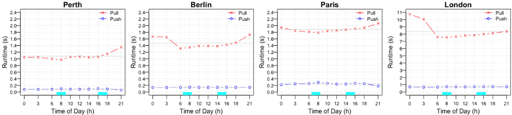
The mean query runtimes for both the baseline pull approach and the proposed push approach are presented in Figure 3.
5 https://openmobilitydata.org
6 https://files.inria.fr/gang/graphs/public transport
7 https://tfl.gov.uk/corporate/publications-and-reports
| Metric | Perth | Berlin | Paris | London |
|---|---|---|---|---|
| Envelope Size | 5.9% | 3.7% | 7.5% | 2.8% |
| Pushed Data (MB) | 1.4 | 1.6 | 4.1 | 4.8 |
| Journey Delayed | 3.7% | 4.8% | 4.2% | 6.0% |
| Envelope Delayed | 73.6% | 81.0% | 94.0% | 87.5% |
| Neither Delayed | 22.7% | 14.2% | 1.8% | 6.5% |
This runtime reflects the average total time required to process a query from the source to the target, including replanning at each intermediate stop along the journey-whether handled solely by the server (pull approach) or shared with the edge device (push approach). The results demonstrate the efficiency of the push approach, achieving runtimes well within a fraction of a second, while the pull approach requires several seconds. The push approach consistently achieves an order-of-magnitude speedup across all datasets and times of day. This translates to the push approach being capable of handling 10 times more queries than the pull approach within the same time period. The relatively slower runtimes for the London dataset are due to its larger number of connections. The pull approach performs worse overnight due to the low frequency of relevant services, especially when a transfer is missed, leading to scanning more unnecessary connections.
Table 2 shows statistics for the push approach across datasets, including the average envelope size and the average percentage of stops per query where delays affect the current journey, the envelope, or neither. Two key factors contribute to the superior performance of the push approach: (i) the significantly smaller size of the envelope compared to the full connections array (around 5%), which considerably reduces the search space, and (ii) the infrequent need for server calls to reconstruct the envelope (about 5% of the intermediate stops). This low frequency means the server receives approximately 20 times fewer calls compared to the pull approach (where a request is made at every stop), enabling a significantly higher query handling capacity. Finally, the statistics indicate that the amount of data sent from the server to each edge device, which represents the total envelope (re)construction and its updates during the journey, is modest, averaging only 3 megabytes. This demonstrates the practicality of the push approach for real-world applications.
5.2 Experiment 2: Arrival Time Saving
To examine travel time savings from dynamic replanning (DR), we develop three alternative baseline strategies for handling disruptions. First, static planning (SP) represents the default strategy, where users plan their journey using the published delay-free timetable and follow the plan as closely as possible despite any delays. If the plan fails due to a missed transfer, users attempt to repair the static plan with minimal deviation. They wait at the same stop and take the next available train to the next transfer stop. Second, in the Snapshot Replanning (SR) strategy, users (re)plan their journey at τq based on the most recent delay updates just before starting from the origin stop, and then react to delays as in static planning. Finally, in the journey-delayed replanning (JDR) strategy, replanning occurs only when the current journey is delayed; essentially removing lines 6-8 from Algorithm 2. JDR can be understood as an improvement on contingent planning, integrating real-time delays and replanning dynamically. For journeys that arrive extremely late in these baselines due to a lack of available services and require waiting until the next day, we assume users will not wait indefinitely before seeking alternative actions (e.g., taking a taxi). In such cases, a penalty of 90 minutes is applied to account for inconvenience and extra time and cost. This means users are considered to arrive only 90 minutes later than they would with DR.
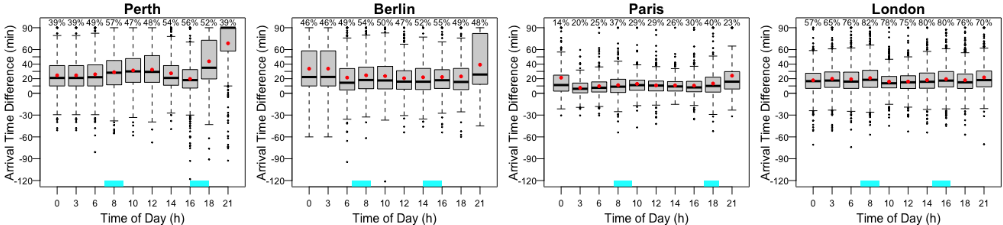
DR vs. SP. Figure 4 illustrates the difference in arrival time at the destination between DR and SP throughout the day, excluding queries with identical arrival time in both scenarios. The results show that a significant portion of journeys are affected, with almost half in both Perth and Berlin, slightly fewer in Paris, and more in London. The mean difference in arrival time for affected journeys ranges from 20 to 30 minutes of time savings in both Perth and Berlin, and from 5 to 20 minutes in both Paris and London. Note that in a few cases (around 4-5% of journeys), DR may result in a later arrival than SP. This occurs when the updated plan advised by DR encounters significant unforeseen delays later. The findings also show that affected journeys during overnight hours (i.e., 0, 3, and 21) are generally fewer but result in larger time savings compared to the rest of the day. This is because services are less frequent during these hours, so even if a journey is delayed, transfers are more likely to remain valid. However, if a transfer is missed, the consequences can be significant, leading to longer waits and late arrivals.
| Comparison | Metric | Perth | Berlin | Paris | London |
|---|---|---|---|---|---|
| DR vs. SR | Q. Affected Avg. Saving | 42.3% 30.2 | 41.1% 24.2 | 20.4% 10.6 | 66.2% 16.0 |
| DR vs. JDR | Q. Affected Avg. Saving | 10.0% 5.7 | 13.1% 4.6 | 13.3% 6.0 | 21.1% 4.9 |
DR vs. SR and JDR. Table 3 shows the advantages of DR compared to both SR and JDR scenarios. SR can provide a limited improvement over SP. Considering JDR, a significant part of the time savings of DR comes from replanning even when the current journey is not even delayed. This demonstrates the importance of the dynamic replanning in minimising the impact of disruptions.
6 Conclusion and FutureWork
We innovatively formulated dynamic replanning in public transport routing to address delays, shifting the initiative from users to the system, which proactively ensures they remain on the best path. This approach demonstrates both query efficiency and travel time savings. It opens several directions for future work, including further improving envelope tightness, developing more selective triggers for envelope-based replanning, testing with real-world delay data, and extending to multicriteria routing (e.g., number of transfers).
Acknowledgements
This work was partially funded by the Australian Research Council (ARC) under grant DP190100013.
@inproceedings{ijcai2025p937,
  title     = {Dynamic Replanning for Improved Public Transport Routing},
  author    = {Abuaisha, Abdallah and Shen, Bojie and Harabor, Daniel D. and Stuckey, Peter J. and Wallace, Mark},
  booktitle = {Proceedings of the Thirty-Fourth International Joint Conference on
               Artificial Intelligence, {IJCAI-25}},
  publisher = {International Joint Conferences on Artificial Intelligence Organization},
  editor    = {James Kwok},
  pages     = {8430--8437},
  year      = {2025},
  month     = {8},
  note      = {Main Track},
  doi       = {10.24963/ijcai.2025/937},
  url       = {https://doi.org/10.24963/ijcai.2025/937},
}
TY - CPAPER TI - Dynamic Replanning for Improved Public Transport Routing AU - Abuaisha, Abdallah AU - Shen, Bojie AU - Harabor, Daniel D. AU - Stuckey, Peter J. AU - Wallace, Mark T2 - Proceedings of the Thirty-Fourth International Joint Conference on Artificial Intelligence, IJCAI-25 PB - International Joint Conferences on Artificial Intelligence Organization PY - 2025 SP - 8430 EP - 8437 DO - 10.24963/ijcai.2025/937 UR - https://doi.org/10.24963/ijcai.2025/937 ER -Copied
Machine-readable versions of this paper, for tools and AI agents:





