Solving MDPs with LTLf+ and PPLTL+ Temporal Objectives

1 Introduction

Temporal logics are widely used as specification languages in reactive synthesis and adversarial planning [Baier and Katoen, 2008; Camacho et al., 2019]. Among these, linear temporal logic (LTL) [Pnueli, 1977] is perhaps the most commonly used. LTL is a formalism used to specify and reason about the temporal behaviour of systems over infinite traces. It has been extensively employed as a specification mechanism for temporally extended goals, as well as for expressing preferences and soft constraints in various fields, including business processes, robotics, and AI [Bienvenu et al., 2011; Maggi et al., 2011; Fainekos et al., 2009]. Linear temporal logic over finite traces (LTLf) [Baier and McIlraith, 2006; De Giacomo and Vardi, 2013; De Giacomo and Vardi, 2015] is a variant of LTL with the same syntax but it is interpreted over finite instead of infinite traces. PPLTL is the pure-past version of LTLf and scans the trace backwards from the end towards the beginning [De Giacomo et al., 2020]. It is wellestablished that strategy synthesis for LTLf and PPLTL can be derived from deterministic finite automata (DFA), thereby avoiding the challenges associated with determinising automata for infinite traces, typical of LTL reactive synthesis.

∗Corresponding author

The temporal logics LTLf+ and PPLTL+ have recently been proposed to express objectives over infinite traces [Aminof et al., 2024]. These logics are directly based on Manna and Pnueli's hierarchy of temporal properties [Manna and Pnueli, 1990]. This hierarchy categorizes temporal properties on infinite traces in four classes, which are obtained by requiring that a finite trace property holds for some prefixes of infinite traces ("guarantee"), all prefixes ("safety"), infinitely many prefixes ("recurrence") and for all but finitely many prefixes ("persistence"). Notably every LTL property can be expressed as a Boolean combination of these four kinds of properties [Manna and Pnueli, 1990]. LTLf+ and PPLTL+ use respectively LTLf and PPLTL to express properties over finite traces and obtain the four basic kinds of infinite trace properties of the Manna and Pnueli's hierarchy. This makes them particularly interesting from the computational point of view. While they retain the expressive power of LTL on infinite traces, they enable the lifting of DFA-based techniques developed for LTLf and PPLTL to obtain deterministic automata on infinite traces corresponding to formulas, thus avoiding determinisation of B¨uchi automata, which is known to be a notorious computational bottleneck. As a result, LTLf+ and PPLTL+ are particularly promising for a number of tasks, such as reactive synthesis [Pnueli and Rosner, 1989; Finkbeiner, 2016], supervisory control for temporal properties [Ehlers et al., 2017], and planning for temporally extended goals in nondeterministic domains [Bacchus and Kabanza, 1998; De Giacomo and Rubin, 2018]. All these determin-

istic automaton on infinite traces, to be used as a game arena over which a strategy can be computed to achieve the required property. LTLf+ and PPLTL+ excel at these tasks by enabling simple arena construction through the Cartesian product of DFAs, corresponding to the finite trace (LTLf/PPLTL) components in the LTLf+/PPLTL+ formula. On the other hand, the game to be solved over this arena is an Emerson-Lei game [Emerson and Lei, 1987], which requires quite sophisticated techniques [Hausmann et al., 2024].

In this paper, we demonstrate that these logics are even more effective in the context of MDPs. Traditionally, deterministic Rabin automata have been the standard choice for representing LTL specifications in MDPs [Baier and Katoen, 2008]. Due to the probabilistic nature of MDPs, the automaton for temporal specifications does not need to be entirely deterministic. State-of-the-art MDP synthesis methods use a restricted form of B¨uchi automata called LimitDeterministic B¨uchi Automata (LDBAs) for LTL [Hahn et al., 2015; Sickert et al., 2016; Shao and Kwiatkowska, 2023]. Recent work has shown that an even more relaxed form of nondeterminism, termed "good for MDPs" (GFM), can be effectively used for MDP synthesis [Hahn et al., 2020; Schewe et al., 2023].

Since this relaxed nondeterminism enables more succinct representations of temporal specifications, we adopt GFM automata in this work. By leveraging GFM's controlled nondeterminism, we present techniques for solving MDPs with LTLf+/PPLTL+ objectives that maintain the compositional DFA-based approach of [Aminof et al., 2024]. Instead of using Emerson-Lei automata, our construction obtains simple LDBAs from the DFAs of LTLf/PPLTL components corresponding to Manna and Pnueli's four classes, then composes them while preserving the "good for MDPs" property. The result is a GFM B¨uchi automaton that can be used to solve MDPs in a standard way [Baier and Katoen, 2008]. This gives us a simple technique that not only is sound, complete, and computationally optimal, but is both implementation-friendly and well-suited for straightforward symbolic implementation.

2 Preliminaries

In the whole paper, we will fix a set of atomic propositions AP. We denote by Σ = 2AP the set of interpretations over AP; Σ is also called the alphabet set. Let Σ∗ and Σω denote the set of all finite and infinite sequences, respectively. The empty sequence is denoted as ϵ and we index a sequence u = a0a1 · · · an · · · from 0. Moreover, we let Σ+ = Σ∗ \{ϵ}. We denote by w[i · · · j] the fragment that starts at position i and ends (inclusively) at position j. Particularly, ϵ = w[i · · · j] for all w if j < i. We denote by |w| the number of letters in w if w is a finite sequence and ∞ otherwise. For a finite or infinite sequence w, w[0 · · · i] is said to be a prefix of w if 0 ≤ i < |w|. A trace is a non-empty finite or infinite sequence of letters in Σ; Specially, ϵ is not a trace.

2.1 LTLf+ and PPLTL+ over Infinite Traces

LTLf+ and PPLTL+ have been derived from LTLf and PPLTL, respectively [Aminof et al., 2024]. The syntax of an LTLf formula [Baier and McIlraith, 2006; De Giacomo and Vardi, 2013] over a finite set of propositions AP is defined as ϕ ::= a ∈ AP | ¬ϕ | ϕ ∧ ϕ | ϕ ∨ ϕ | Xϕ | ϕUϕ | Fϕ | Gϕ. Here X (strong Next), U (Until), F (or ⋄) (Finally/Eventually), and G (or □) (Globally/Always) are temporal operators. The syntax of Pure Past LTL over finite traces (PPLTL) is given as ϕ ::= a ∈ AP | ¬ϕ | ϕ∧ϕ | ϕ∨ϕ | Yϕ | ϕSϕ. Here Y ("Yesterday") and S ("Since") are the past operators, analogues of "Next" and "Until", respectively, but in the past.

Although LTLf and PPLTL have the same expressive power, translating LTLf to DFAs requires a doubly exponential blow-up [De Giacomo and Vardi, 2013], while translating PPLTL to DFAs requires only a singly exponential blowup [De Giacomo et al., 2020]. We refer interested readers to [De Giacomo and Vardi, 2013] and [De Giacomo et al., 2020] for the semantics of LTLf and PPLTL, respectively. The language of an LTLf/PPLTL formula ϕ, denoted [ϕ], is the set of finite traces over 2AP that satisfy ϕ.

The syntax of LTLf+ (resp. PPLTL+) is given by the following grammar:

where ϕ are finite-trace formulas in LTLf/PPLTL over AP.

Let w ∈ Σω be an infinite trace and ϕ an LTLf/PPLTL formula. We use |=+ for non-empty finite traces and |= for infinite traces. The semantics of an LTLf+/PPLTL+ formula is defined by quantifying over the prefixes of infinite traces:

• w |= ∀ϕ means that, for all i ≥ 0, w[0 · · · i] |=+ ϕ.
• w |= ∀∃ϕ means that, for every i ≥ 0, there exists an integer j ≥ i such that w[0 · · · j] |=+ ϕ.
• w |= ∃ϕ means that there exists an integer i ≥ 0 such that w[0 · · · i] |=+ ϕ.
• w |= ∃∀ϕ means that there exists an integer i ≥ 0 such that, for all integer j ≥ i, w[0 · · · j] |=+ ϕ.

Similarly, we denote by [Ψ] the set of infinite traces satisfying the LTLf+/PPLTL+ formula Ψ. It has been shown in [Aminof et al., 2024] that LTLf+, PPLTL+, and LTL have the same expressive power.

2.2 Markov Decision Processes

Following [Baier and Katoen, 2008], a Markov decision process (MDP) M is a tuple (S,Act, P, s0, L) with a finite set of states S, a set of actions Act, a transition probability function P : S × Act × S → [0, 1], an initial state s0 ∈ S and a labelling function L : S → 2AP that labels a state with a set of propositions that hold in that state. A path ξ of M is a finite or infinite sequence of alternating states and actions ξ = s0a0s1a1 · · · , ending with a state if finite, such that for all i ≥ 0, ai ∈ Act(si) and P(si, ai, si+1) > 0. The sequence L(ξ) = L(s0)L(s1), · · · over AP is called the trace induced by the path ξ over M.

A strategy σ of M is able to resolve the nondeterminism of an MDP and induces a Markov chain (MC) Mσ = (S+, Pσ, AP, L′ ) where for u = s0 · · · sn ∈ S+, Pσ(u, u · sn+1) = P(sn, σ(u), sn+1) and L′ (u) = L(sn).

Denote by FPaths and IPaths the set of all finite and infinite paths of M, respectively. A strategy σ of M is a function σ : FPaths → Distr(Act) such that, for each ξ ∈ FPaths, σ(ξ) ∈ Distr(Act(lst(ξ))), where lst(ξ) is the last state of the finite path ξ and Distr(Act) denotes the set of all possible distributions over Act. Let ΩMσ (s) denote the subset of (in)finite paths of M that correspond to strategy σ and initial state s0.

A sub-MDP of M is an MDP M′ = (S′ ,Act′ , P′ , L) where S′ ⊆ S,Act′ ⊆ Act is such that for every s ∈ S′ , Act′ (s) ⊆ Act(s), and P′ and L′ are obtained from P and L, respectively, when restricted to S′ and Act′ . In particular, M′ is closed under probabilistic transitions, i.e., for all s ∈ S′ and a ∈ Act′ we have that P′ (s, a, s′ ) > 0 implies that s′ ∈ S′ . An end-component (EC) of an MDPM is a sub-MDPM′ of M such that its underlying graph is strongly connected and it has no outgoing transitions. A maximal end-component (MEC) is an EC E = (E,Act′ , P′ , L) such that there is no other EC E = (E′ , Act′′ , P′′ , L) such that E ⊂ E′ . An MEC E that cannot reach states outside E is called a leaf component.

Theorem 1 ([de Alfaro, 1997; Baier and Katoen, 2008]). Once an end-component E of an MDP is entered, there is a strategy that visits every state-action combination in E with probability 1 and stays in E forever. Moreover, for every strategy the union of the end-components is visited with probability 1. An infinite path of an MCM almost surely (with probability 1) will enter a leaf component.

2.3 Automata

A (nondeterministic) transition system (TS) is a tuple T = (Q, q0, δ), where Q is a finite set of states, q0 ∈ Q is the initial state, and δ : Q×Σ → 2Q is a transition function. We also lift δ to sets as δ(S, a) := ⋃q∈S δ(q, a). A deterministic TS is such that if, for each q ∈ Q and a ∈ Σ, |δ(q, a)| ≤ 1.

An automaton A is defined as a tuple (T , α), where T is a TS and α is an acceptance condition. A finite run of A on a finite word u of length n ≥ 0 is a sequence of states ρ = q0q1 · · · qn ∈ Q+ such that, for every 0 ≤ i < n, qi+1 ∈ δ(qi, u[i]), where u[i] indicates the letter of u in position i.

For finite words, we consider finite automata with deterministic TS, known as deterministic finite automata (DFA), where α = F ⊆ Q is a set of final states. A finite word u is accepted by the DFA A if its run q0 · · · qn ends in a final state qn ∈ F. For an infinite word w, a run of A on w is an infinite sequence of states ρ = q0q1q2 · · · such that, for every i ≥ 0, qi+1 ∈ δ(qi,w[i]). Let inf(ρ) be the set of states that occur infinitely often in the run ρ. We consider the following acceptance conditions for automata on infinite words:

B¨uchi/co-B¨uchi. α = F ⊆ Q is a set of accepting (rejecting, resp.) states for B¨uchi (co-B¨uchi, resp.). A run ρ satisfies the B¨uchi (co-B¨uchi, resp.) acceptance condition α if inf(ρ) ∩ F ̸= ∅ (inf(ρ) ∩ F = ∅, resp.).

Rabin. α = ⋃ki=1 {(Bi,Gi)} is such that Bi ⊆ Q and Gi ⊆ Q for all 1 ≤ i ≤ k. A run ρ satisfies α if there is some j ∈ [1, k] such that inf(ρ)∩Gj ̸= ∅ and inf(ρ)∩Bi = ∅.

A run is accepting if it satisfies the condition α; A word w ∈ Σω is accepted by A if there is an accepting run ρ of A over w. We use three letter acronyms in {D,N} × {F, B, C, R} × {A} to denote automata types where the first letter stands for the TS mode, the second for the acceptance type and the third for automaton. For instance, DBA stands for deterministic B¨uchi automaton. An NBA is called a limit deterministic B¨uchi automaton (LDBA) if its TS becomes deterministic after seeing accepting states in a run. We assume that all automata are complete, i.e., for each state s ∈ Q and letter a ∈ Σ, |δ(s, a)| ≥ 1.

We denote by L∗(A) the set of finite words accepted by a DFA A or the language of A. Similarly, we denote by L(A) the ω-language recognized by an ω-automaton A, i.e., the set of ω-words accepted by A.

3 Classic MDP Synthesis Approach

In non-probabilistic scenarios, such as reactive synthesis and planning, deterministic ω-automata have to be constructed, e.g. [Aminof et al., 2024]. In contrast, in the probabilistic setting, there can be a controlled form of nondeterminism called good for MDPs (GFM) due to the effect of probabilities [Hahn et al., 2020; Schewe et al., 2023]. More precisely, to synthesise a strategy σ for an MDP M that maximises the satisfaction probability of a given temporal objective Ψ, we do the following steps: first, we construct a GFM automaton A that recognises [Ψ], then build the product MDPM×A, and finally synthesise a strategy σ on M×A that maximises the probability of reaching accepting MECs. Our MDP synthesis algorithm with LTLf+ and PPLTL+ objectives follows the same methodology; our main contribution is a construction of LTLf+/PPLTL+ to GFM automata.

To make our presentation more general, we will assume that we are given a (possibly nondeterministic) ω-automaton A = (Q, δ, q0, α) as specification and an MDP M = (S, Act, P, s0, L). To find an optimal strategy σ, we define the semantic satisfaction probability of the induced MCMσ for L(A) as PMσ(L(A)) = P{ξ ∈ ΩMσ (s0) : L(ξ) ∈ L(A)}.

For an MDP M, we define the maximal semantic satisfaction probability as Psem(M,A) = supσ PMσ(L(A)). Clearly, for two language-equivalent automata A and B, it holds that Psem(M, A) = Psem(M, B).

Product MDP. As aforementioned, we find the strategy that obtains Psem(M, A) by building M× A, formally defined as M × A = (S × Q, Act × Q, P×, ⟨s0, q0⟩, L×, α×) augmented with the acceptance condition α× where

• P× : (S×Q)×(Act×Q)×(S×Q) → [0, 1] such that P×(⟨s, q⟩, ⟨a, q′ ⟩, ⟨s′ , q′ ⟩) = P(s, a, s′ ) if P(s, a, s′ ) > 0 and q′ ∈ δ(q, L(s)),
• For B¨uchi/co-B¨uchi, α× = F × = {⟨s, q⟩ ∈ S × Q : q ∈ F}, while for Rabin, B× i = {⟨s, q⟩ : q ∈ Bi} and G×i = {⟨s, q⟩ : q ∈ Gi} for i ∈ [1, k].
• L×(⟨s, q⟩) = L(s) for a state ⟨s, q⟩ ∈ S ×Q, and

Intuitively, M× A resolves the nondeterminism in A by making each successor an explicit action. Then, we can generate traces in L(A) by enforcing the acceptance condition α. Now we define the maximal syntactic satisfaction probability: Psyn(M, A) = sup σ P{ξ ∈ ΩM×A σ (⟨s0, q0⟩) : ξ is accepting}.

Clearly, Psyn(M,A) ≤ Psem(M,A) because accepting runs ξ only occur on accepting words. Moreover, Psyn(M, A) = Psem(M, A) if A is deterministic.

An EC containing an infinite run that visits all states and transitions yet satisfies α× is said to be accepting. According to Theorem 1, all state-action pairs in an EC can be visited with probability 1. Since an accepting run of M×A must eventually enter an accepting MEC [Baier and Katoen, 2008], the syntactic satisfaction probability can be formalised as:

where X is the set of states of the accepting MECs (AMECs) in M× A. GFM automata are the ω-automata, whose nondeterminism can be correctly resolved by the strategy. Formally, An ω-automaton A is GFM if, for all finite MDPs M, Psem(M, A) = Psyn(M, A) holds [Hahn et al., 2020].

Typical GFM automata include: i) deterministic automata, ii) good-for-games automata [Henzinger and Piterman, 2006] that have a strategy to produce an accepting run for every accepting word, and iii) LDBAs that satisfy certain conditions [Hahn et al., 2015; Sickert et al., 2016].

To use GFM automata in synthesis, we describe a gametheoretic approach to decide what automata are GFM.

AEC-simulation game. While determining the GFMness of an NBA is PSPACE-hard [Schewe et al., 2023], we can use the two-player accepting end-component simulation (AEC simulation) game [Hahn et al., 2020] between Spoiler and Duplicator to prove that our constructed automata are GFM. Specially, given a GFM automaton A and an automaton B with L(B) = L(A), if Duplicator wins the AEC-simulation game, B is also GFM.

Theorem 2 ([Hahn et al., 2020]). If A is GFM, B AECsimulates A and L(B) = L(A), then B is also GFM.

In the game, Spoiler places a pebble on the initial state of A, and Duplicator responds by placing a pebble on the initial state of B. The players moves alternately: Spoiler chooses a letter and transition in A, and Duplicator chooses the corresponding transition over the same letter in B. Unlike classic simulation games, Spoiler can, once during the game, make an AEC claim, that she has reached an AEC and provide all transition sequences that will henceforth occur infinitely often in A. Those transitions cannot be updated afterwards. The game continues with both players producing infinite runs in their respective automata. Duplicator wins if: (1) Spoiler never makes an AEC claim, (2) the run constructed in B is accepting, (3) the run constructed in A does not comply with the AEC claim, or (4) the run constructed in A is not accepting. We say that B AEC-simulates A, if Duplicator wins.

The intuition behind Theorem 2 is that, for any MDPM, by Theorem 1, an accepting run of M× A eventually enters an AMEC with probability 1, and the transitions infinitely visited in that AMEC are fixed. When Spoiler makes the AEC claim as the run enters the AMEC, Duplicator can select an accepting run inM×B based on the fixed list of finite traces. Hence, Psyn(M, B) ≥ Psyn(M, A). Since L(A) = L(B) and A is GFM, we have Psyn(M, B) ≥ Psyn(M,A) = Psem(M,A) ≥ Psem(M, B). The key idea is that, once an AMEC is entered, the list of infinitely visited transitions is fixed due to probability, unlike in the usual simulation game.

GFM automata are more succinct than deterministic automata [Sickert et al., 2016; Schewe and Tang, 2023]. This then means that we can obtain smaller product MDP M× A with GFM automata and thus a smaller strategy σ since σ uses the states inM×A as memory.

We now give a useful observation to prove that our constructed automata from LTLf+/PPLTL+ are GFM. It basically says that language equivalent GFM automata can AECsimulate each other when an MC is given. Our proof idea is simple: we just use the optimal strategy σ of M× B that obtains Psem(M, B) for Duplicator to play against Spoiler. In this way, Duplicator can always win the AEC-simulation game because Psem(M, A) = Psem(M, B).

b

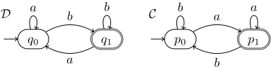
Figure 1: The example DFA D for LTLf formula ϕ := F(last ∧ good) that accepts a finite trace in which the proposition good holds at the last position, and the DFA C for the language [¬ϕ]. Here last indicates the last position of a finite trace, i.e., last := ¬(Xtrue) and Σ := 2AP = {a := ¬good, b := good}.

Theorem 3. Let A and B be two GFM automata such that L(A) = L(B). For any MC M, there is a strategy σ for M × B to AEC-simulate M × A.

With these preparations, we present our synthesis approach: Section 4 covers LTLf+/PPLTL+ to GFM automata, and Section 4.3 outlines our synthesis method.

4 LTLf+/PPLTL+ to GFMB¨uchi Automata

For a given LTLf+/PPLTL+ formula Ψ, we first construct DFAs for its LTLf/PPLTL subformulas, followed by automata operations to derive the final GFM automaton. Existing constructions of GFM LDBAs [Hahn et al., 2015; Sickert et al., 2016] and GFM NBAs [Hahn et al., 2020] from LTL rely on formula unfolding and construct an explicit state automaton without minimisation. 1 In contrast, our approach has two key advantages: First, it leverages efficient DFA-based techniques including minimisation at every intermediate step; Second, it employs a compositional methodology where the automata for subformulas are constructed and optimised independently before being combined, rather than working with the formula as a whole. Moreover our construction can exploit symbolic techniques. These aspects allow us to better handle complex specifications by controlling state space growth throughout the process. This approach applies to PPLTL [De Giacomo et al., 2020].

We assume that we have a construction at hand to efficiently build the DFA for a given LTLf/PPLTL formula ϕ. More precisely, we denote by DFA(ϕ) the DFA constructed for ϕ. Note that, DFA(ϕ) does not accept the empty sequence ϵ by definition 2 . Figure 1 shows a DFA for the LTLf formula ϕ := F(last ∧ good), alongside a DFA for the language [¬ϕ].

4.1 Construction for ∃ϕ, ∀ϕ, ∀∃ϕ, and ∃∀ϕ

Next we describe the GFM automata constructions of the formulas ∃ϕ, ∀ϕ, ∀∃ϕ and ∃∀ϕ, which we call leaf formulas.

∃ϕ. We first present the construction for ∃ϕ below.

1. First, let D = (Σ,Q, ι, δ, F) be DFA(ϕ) such that L∗(D) = [ϕ].

1 For a discussion on minimisation on automata on infinite words, see [Schewe, 2010].

2 In some literature, ϵ ∈ [ϕ] is allowed. In this situation, we must make sure that L∗(DFA(ϕ)) = Σ+ ∩ [ϕ] since the evaluation of the satisfaction for the LTLf+ and PPLTL+ formulas quantifies over nonempty finite traces of the infinite trace.

1. Second, make all final states in F sink final states, i.e., δ(s, a) = s for each s ∈ F and a ∈ Σ, obtaining the automaton C = (Q, ι′ , δ′ , F ′ ). C remains deterministic.

1. Finally, read it as DBA B = (Q, ι′ , δ′ , F ′ ).

By making final states sink, every word accepted in B must have a prefix belonging to [ϕ]. Hence, the theorem follows.

∀ϕ. Nowwe introduce the construction for ∀ϕ.

1. Then, make all final states in C as sink final states, remove unreachable states and obtain the DFA C ′ = (Q′ , ι, δ′ , F ′ )
2. First, let C = (Q, ι, δ, F) be DFA(¬ϕ) such that L∗(C) = [¬ϕ].
3. Finally, reverse the set of final states and read it as B¨uchi automaton B = (Q′ , ι, δ′ , Q′ \ F ′ ).

By making final states of C sink states, every accepting run over a word w in B does not visit those sink final states in C, which then entails that no prefixes of w belong to [¬ϕ]. That is, all prefixes of w belong to ϕ. Then the theorem follows. Our construction for ∀ϕ is quite similar to the one in [Bansal et al., 2023].

∀∃ϕ. The construction for ∀∃ϕ is simple and given below.

1. Then, read D as B¨uchi automaton B = (Q, ι, δ, F).
2. First, let D = (Q, ι, δ, F) be the DFA DFA(ϕ).

Theorem 6 clearly holds since every accepting run in B has a finite prefix run that is an accepting run in D. Figure 2 shows the B¨uchi automata constructed for ∃ϕ, ∀ϕ and ∀∃ϕ.

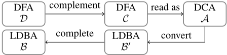
∃∀ϕ. The construction for ∃∀ϕ is more involved and the flowchart is depicted below. The idea is to first build the DCA A for ∃∀ϕ, which is also the DBA for ∀∃¬ϕ and then convert A to the desired LDBA B accepting [∃∀ϕ]. In detail:

B

B′

1. First, complement D by reversing the set of final states, and obtain the DFA C = (Q, ι, δ, Q \ F ) for ¬ϕ.
2. Second, read C as a co-B¨uchi automaton A = (Q, ι, δ,Q \ F). If we treat C as a B¨uchi automaton G, by Theorem 6, L(G) = L(∀∃¬ϕ). Since A is dual to G, we immediately have L(A) = Σω \ L(G) = L(∃∀ϕ).
3. Third, convert A to a LDBA B′ = (Q × {0, 1}, ⟨ι, 0⟩, δ′′ , F × {1}) where δ′′ = δ0 ⊎ δj ⊎ δ1 is defined as follows:
4. ⟨q′ , 0⟩ = δ0(⟨q, 0⟩, a) for all q ∈ Q, q′ ∈ Q and a ∈ Σ with δ(q, a) = q′ ,
5. ⟨q′ , 1⟩ = δj(⟨q, 0⟩, a) for all q ∈ Q, q′ ∈ F and a ∈ Σ with δ(q, a) = q′
6. ⟨q′ , 1⟩ = δ1(⟨q, 1⟩, a) for all q ∈ F, q′ ∈ F and a ∈ Σ with δ(q, a) = q′ ,
7. Finally, complete the LDBA B′ and obtain the result B = (Q′ , ι, δ′ , F ′ = F × {1}).

An accepting run of G must visit Q \ F infinitely often; equivalently, an accepting run of A must visit only F-states from some point on. The intuition behind the NBA B′ is that it has to guess that point via the transition δj. Thus, before that point, B′ stays within the component Q× {0}, and once the run of B′ has entered the component F × {1} via δj, it visits only states in F × {1} from that moment forward.

While the DBAs for ∀ϕ and ∃ϕ can be minimized in polynomial time [L¨oding, 2001], minimizing the ones for ∀∃ϕ and ∃∀ϕ can be NP-complete [Schewe, 2010]. Nonetheless, we can apply cheaper reduction operations such as extreme minimisation [Badr, 2009] to B.While the construction gives a LDBA instead of DBAs, the resulting LDBA is also GFM.

Theorem 8. The automata B for each of ∃ϕ, ∀ϕ, ∀∃ϕ, and ∃∀ϕ are GFM.

Proof. In fact we have seen that the automaton B for ∃ϕ, ∀ϕ, ∀∃ϕ is a DBA so trivially GFM. We prove the result for the automaton B for ∃∀ϕ by creating an AEC-simulation game between Spoiler and Duplicator. Spoiler will play on DCA A and Duplicator will play on B. First, L(A) = L(B) = [∃∀ϕ]. Moreover, A is a GFM automaton because A is deterministic. Therefore, if we can prove that B AECsimulates A, then B is also GFM according to theorem 2.

Now we provide a winning strategy for Duplicator on B in the AEC-simulation game. Before Spoiler makes the AEC claim, Duplicator will take transitions within Q× {0} via δ0. Once the AEC claim is made by Spoiler, the Duplicator will transition to F × {1} via δj at the earliest point. Afterwards, Duplicator takes transitions within F × {1} via δ1. The only situation where Spoiler wins is that the run ρ in A over the chosen word w is accepting. That is, ρ cannot visit Q \ F states any more after the AEC claim since the list of finite traces visited infinitely often is fixed. This then entails that the run ̂ ρ constructed by Duplicator will also be accepting in B since the projection on Q of ̂ ρ is exactly ρ. It follows that Duplicator wins the game and B AEC-simulates A. Hence, B is also GFM according to Theorem 2.

Following example, illustrates why the constructed LDBA B for ∃∀ϕ is GFM.

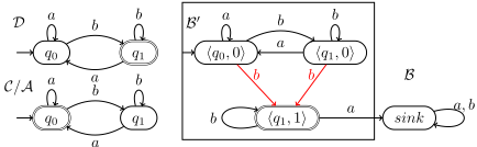
Example 1. Consider the DFA D for ϕ on the upper left of Figure 3. The DCA A (or DFA C) with rejecting states {q0} is shown on the lower left, and the complete LDBA B is on the right (LDBA B′ is within the dashed box). The

a

Figure 3: The DFA D for ϕ is on upper left, the DCA A (or DFA C) with the set of rejecting states {q0} is on lower left, A has language {a, b}∗ · bω and the LDBA B′ is the part within the dashed box and B is the complete LDBA where {⟨q1, 1⟩} is the sole accepting state marked with double rounded boxes and the jump transitions in δj are drawn in red colour.

sole accepting state {⟨q1, 1⟩} is marked with double rounded boxes, and jump transitions in δj are in red. A winning strategy for the Duplicator allows B to AEC-simulate A. Let δ and δ′ be the transition functions of A and B, respectively. The strategy σ works as follows: (1) Before the AEC-claim, σ(u) = δ′ (⟨q0, 0⟩, u); (2) At the AEC claim, σ takes the jump transition upon reading b as soon as possible; (3) Afterwards, σ uses δ′ for successors. The Spoiler can win only by making an AEC claim and forcing A to stay in q1 forever. In this case, σ ensures an accepting run.

4.2 Boolean Combinations of GFMAutomata

Now, we show that GFM automata are closed under union and intersection. Let A0 and A1 be two GFM B¨uchi automata. First we introduce the union operation for A0 and A1.

This union operation is just a Cartesian product of A0 and A1. Let w ∈ Σ∗ . For the word w, a run ρ0 of A0 and a run ρ1 of A1 constitute a run A in the form of ρ0 ×ρ1. So, if one of the runs is accepting, ρ0 × ρ1 is also accepting. We show below that the union automaton is also GFM.

Proposition 1. Given two B¨uchi automata A0 = (Q0, ι0, δ0, F0) and A1 = (Q1, ι1, δ1, F1), let A = (Q, ι, δ, F) be the B¨uchi automaton where Q = Q0 × Q1, ι = (ι0, ι1), δ(⟨q0, q1⟩, a) = δ0(q0, a) × δ1(q1, a), and F = Q0 × F1 ∪ F0 × Q1. Then, L(A) = L(A0) ∪ L(A1) with |Q| = |Q0| · |Q1|.

Theorem 9. If A0 and A1 are both GFM, then the union automaton A is also GFM.

Proof. Let M = (S,Act, P, s0, L) be an MDP. Our proof goal is to show that Psyn(M,A) = Psem(M,A). Then, we can just prove that Psyn(M,A) ≥ Psem(M,A). We will prove it with the help of equivalent DRAs of A0 and A1.

Let R0 = (Q′0 , δ′0 , ι′0 , α′0 ) and R1 = (Q′1 , δ′1 , ι′1 , α′1 ) be two DRAs that are language-equivalent to A0 and A1, respectively. Let R = R0 × R1 be the union DRA of R0 and R1 such that L(R) = L(R0) ∪ L(R1). Formally, R is a tuple (Q′ = Q′0 × Q′1 , δ′ , ι′ = ⟨ι′0 , ι′1 ⟩, α′ ) where δ′ (⟨q0, q1⟩, a) = ⟨δ′0 (q0, a), δ′1 (q1, a)⟩ for each ⟨q0, q1⟩ ∈ Q′ and a ∈ Σ, and α′ = ⋃k0 i=1 {(Bi×Q′1 ,Gi×Q′1 ) : (Bi,Gi) ∈ α′0 } ∪ ⋃k1 i=1 {(Q′0 × Bi,Q′0 × Gi) : (Bi,Gi) ∈ α′1 }. Let w ∈ Σω , and ρ0 and ρ1 are the runs over w in R0 and R1, respectively. The run of R = R0 × R1 over w is actually the product ρ0 × ρ1. Moreover, if w ∈ L(A), then the run

ρ0 ×ρ1 satisfies either α′0 or α′1 , which indicates that ρ0 ×ρ1 is accepting in R. Then, it follows that Psem(M,R) = Psem(M, A) as L(A) = L(R). As R is deterministic, we have Psem(M,R) = Psyn(M,R). Therefore, we only need to prove that Psyn(M, A) ≥ Psyn(M, R).

Let σ be the optimal strategy on M to obtain the maximal satisfaction probability for L(A), i.e.,

Note again that here σ is usually not a positional strategy for M and needs extra memory to store history traces.

We denote by T0, T1 and T0 × T1 the TSes of R0, R1, and R respectively. We now work on the large Markov chain M′ = Mσ × T0 × T1 by ignoring the acceptance conditions where Mσ is already an MC. Thus, M′ has only probabilistic choices. Since R = R0 ×R1 is deterministic, we have that

Let c ∈ {0, 1}. We know that Ac is GFM. According to Theorem 3, there is an optimal strategy σc for M′ × Ac to AEC-simulateM′×Rc. Thus, we construct the optimal strategy σ∗ for M×A by building the product of three strategies σ for M, σ0 and σ1, which resolves the nondeterminism of M, A0 and A1, respectively, independently inM′ ×A (viewing A as the cross product of A0 and A1). That is, in this case, σc works independently from σ1-c on Mσ × T0 × T1 × Ac and the state space of T0 × T1 will be used as extra memory for σc in addition to store states fromMσ and Ac.

Then, in the AEC-simulation game, whenever Spoiler produces an accepting run in M′ × R, we can use σ∗ to construct an accepting run for Duplicator in M′ ×A0 ×A1 = M′ × A. So, there is a strategy σ∗ on M× A to achieve Psyn(M,A) = Psyn(M′ ,A) ≥ Psyn(M′ ,R). It then follows that Psyn(M,A) ≥ Psyn(M′ ,R) = Psem(M,A). That is, Psyn(M,A) = Psem(M,A) for any given MDP M. Therefore, A is also GFM.

We illustrate why the union product A is GFM if both A0 and A1 are GFM with an example.

The Cartesian product is necessary for A being GFM. The normal union product only adds an extra initial state to nondeterministically select one of the two automata for the subsequent run, which has only |Q1| + |Q2| + 1 states. However, the product might produce an automaton that is not GFM [Schewe et al., 2023].

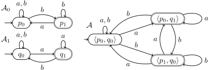
Example 2. Consider the GFM NBAs A0 and A1 on the left of Figure 4, and their union product A on the right. A0 accepts ({a, b}∗ · b)ω , and A1 accepts ({a, b}∗ · a)ω . Both are GFM as they have strategies to generate an accepting run for every accepting word. The winning strategy stays in the initial state before the AEC-claim and then aims to visit the accepting state repeatedly. The union product A is also GFM, with a strategy σ enabling the Duplicator to win the AECsimulation game against any deterministic automaton D. The strategy σ works as follows: Before the AEC claim, σ keeps the run in the initial state ⟨p0, q0⟩. After the AEC claim, σ exits ⟨p0, q0⟩ and confines the run to {⟨p0, q1⟩, ⟨p1, q0⟩}. For any accepting infinite word chosen by the Spoiler, σ ensures an accepting run. In fact, σ combines the winning strategies of A0 and A1. Hence, A is GFM.

b

Figure 4: The GFM NBAs A0 and A1 are depicted on the left and their union product A is depicted on the right. The accepting states are marked with double rounded boxes.

Next, we introduce the intersection operation for the GFM automata and show that the result automaton is also GFM.

Proposition 2 ([Kupferman, 2018]). Given two B¨uchi automata A0 = (Q0, ι0, δ0, F0) and A1 = (Q1, ι1, δ1, F1), let A = (Q, ι, δ, F) be the intersection B¨uchi automaton whose components are defined as follows:

• Q = Q0 × Q1 × {0, 1};
• ι = (ι0, ι1, 0);
• For a state ⟨q0, q1, c⟩ and letter a ∈ Σ, we have ⟨q′0 , q′1 , next(q0, q1, c)⟩ ∈ δ(⟨q0, q1, c⟩, a) where q′0 ∈ δ0(q0, a), q′1 ∈ δ1(q1, a), next : Q0 × Q1 × {0, 1} → {0, 1} is defined as

• F = F0 ×Q1 ×{0}.

This intersection construction is fairly standard [Kupferman, 2018]. The intuition is to alternatively look for accepting states from A0 when c is set to 0 and for accepting states in A1 when c is 1. In this way, the accepting run of A must visit accepting states from both A0 and A1 infinitely often. The resulting automaton is an LDBA.

Similarly, we show that the GFM automata are also closed under the intersection operation by Theorem 10.

Theorem 10. If A0 and A1 are GFM, then the intersection automaton A is also GFM.

In [Hahn et al., 2020], the constructed GFM automata are slim in the sense that each state has at most two successors over a letter. The GFM automata we produce can easily be made slim. This is because the only nondeterministic decision we have to make is to guess in the intersection operation when the individual DCAs will henceforth see only accepting states. This decision can obviously be arbitrarily delayed. We can therefore make them round-robin, considering only one LDBA that stems from a DCA at a time. For instance, when we have positive Boolean operations that contain 42 automata from ∃∀ϕ formulas, then we can avoid the outdegree from jumping to 242 at the expense of increasing the state space by a factor of 42 (while retaining the out-degree of 2) to handle the round-robin in the standard way.

By applying the constructions of B¨uchi automata for leaf formulas and constructions for intersection and union operations on the syntax tree of a LTLf+ or PPLTL+ formula, we can obtain a final B¨uchi automaton for the formula. Therefore, the following result holds.

Theorem 11. For an LTLf+/PPLTL+ formula Ψ, our method constructs a GFM B¨uchi automaton A such that L(A) = [Ψ].

Let |Ψ| be the length of the formula, i.e., the number of modalities and operations in the formula. Then we have that:

Theorem 12. For an LTLf+ (respectively, PPLTL+) formula Ψ, the number of states in A is 22O(|Ψ|) (respectively 2O(|Ψ|) ).

The number of states obtained in Theorem 12 is optimal, in the sense that the worst-case double exponential blow-up (single exponential blow-up) is already unavoidable for LTLf (resp. PPLTL) [Bansal et al., 2023; De Giacomo et al., 2020].

4.3 Returning the Strategy

Given an LTLf+/PPLTL+ formula Ψ and an MDP M, our construction can obtain an optimal strategy for M to achieve maximal satisfaction probability of Ψ as follows.

First, construct a GFM B¨uchi automaton A for Ψ using approaches described in Section 4 with L(A) = L(Ψ).

Second, construct the product M× = M×A and compute the list of AMECs E = {E1, · · · , Ek} inM× using the standard approach described in [Baier and Katoen, 2008].

Finally, synthesise a strategy as follows: In the AMECs, we can select an action for every state that gives the shortest path to the set of accepting states. This shortest path can be multiple but we only need one and the definition of shortest path is clearly well defined. For states outside AMECs, we select an action for every state to reach an AMEC with maximal probability; this is equivalent to computing the strategy for obtaining the maximal reachability probability to AMECs. The resultant strategy, denoted by σ×, is positional on M× for B¨uchi acceptance condition according to [Mazala, 2001].

Since the B¨uchi automaton A for Ψ is GFM we get:

Theorem 13. The synthesised strategy σ× for M is optimal to achieve maximal satisfaction probability of Ψ.

5 Conclusion

In this paper, we investigated the problem of solving MDPs with LTLf+ and PPLTL+ temporal objectives, showing the effectiveness of these logics for probabilistic planning in MDPs. Our key contribution lies in presenting a provably correct technique to construct GFM B¨uchi automata for LTLf+ and PPLTL+ formulas, leveraging the compositional advantages of DFA-based methods. Note that our construction is designed to be implementation-friendly and well-suited for a straightforward symbolic implementation. In fact, for PPLTL we can directly construct the symbolic DFA in polynomial time [De Giacomo et al., 2020]. The final Boolean combination of these symbolic B¨uchi automata, as described in Section 4.2, is at most polynomial in their combined sizes and can be realised through a Cartesian product. As a future work, we aim to implement this approach, employing symbolic techniques, within state-of-the-art tools such as PRISM [Kwiatkowska et al., 2011]. This development will facilitate the practical application of our methods across a range of domains, including AI, robotics, and probabilistic verification.

Acknowledgements

This work has been partially supported by ISCAS Basic Research (Grant Nos. ISCAS-JCZD-202406, ISCAS-JCZD202302), CAS Project for Young Scientists in Basic Research (Grant No. YSBR-040), ISCAS New Cultivation Project ISCAS-PYFX-202201, the ERC Advanced Grant WhiteMech (No. 834228), the UKRI Erlangen AI Hub on Mathematical and Computational Foundations of AI, and the EPSRC through grants EP/X03688X/1 and EP/X042596/1.