
Fast and Stronger Lower Bounds for Planar Euclidean Shortest Paths
Proceedings of the Thirty-Fourth International Joint Conference on Artificial Intelligence. Main Track. Pages 8510-8517.
https://doi.org/10.24963/ijcai.2025/946
Keywords
- Planning and Scheduling: PS: Routing
- Search: S: Combinatorial search and optimisation
- Search: S: Applications
Abstract
We consider the problem of quickly providing strong lower bounds for the planar Euclidean shortest path (ESP) problem. Such lower bounds are crucial for guiding the search in A* type approaches or for proving quality guarantees for algorithms that compute approximate solutions.
Our contributions are two-fold: we show how to simplify ESP instances such that computing and storing a visibility graph becomes feasible while distances within the simplified instance are guaranteed to constitute lower bounds for the original problem instance. Furthermore we show how to precompute a space efficient data structure that allows to perform distance queries on visibility graphs within few microseconds with negligible space overhead.
- [Abraham et al., 2012] Ittai Abraham, Daniel Delling, An- drew V. Goldberg, and Renato Fonseca F. Werneck. Hier- archical hub labelings for shortest paths. In ESA, volume 7501 of Lecture Notes in Computer Science, pages 24-35. Springer, 2012.
- [Aleksandrov et al., 2000] Lyudmil Aleksandrov, Anil Ma- heshwari, and Jörg-Rüdiger Sack. Approximation algo- rithms for geometric shortest path problems. In STOC, pages 286-295. ACM, 2000.
- [Bast et al., 2016] Hannah Bast, Daniel Delling, Andrew V. Goldberg, Matthias Müller-Hannemann, Thomas Pajor, Peter Sanders, Dorothea Wagner, and Renato F. Werneck. Route planning in transportation networks. In Algorithm Engineering, volume 9220 of LNCS, pages 19-80. 2016.
- [Canny and Reif, 1987] John F. Canny and John H. Reif. New lower bound techniques for robot motion planning problems. In FOCS, pages 49-60. IEEE Computer Soci- ety, 1987.
- [Chew, 1989] L. Paul Chew. Constrained delaunay triangu- lations. Algorithmica, 4(1):97-108, 1989.
- [Cohen et al., 2003] Edith Cohen, Eran Halperin, Haim Ka- plan, and Uri Zwick. Reachability and distance queries via 2-hop labels. SIAM J. Comput., 32(5):1338-1355, 2003.
- [Cui et al., 2017] Michael Cui, Daniel Damir Harabor, and Alban Grastien. Compromise-free pathfinding on a navi- gation mesh. In IJCAI, pages 496-502. ijcai.org, 2017. IJCAI
- [Delling et al., 2013] Daniel Delling, Andrew V. Goldberg, Andreas Nowatzyk, and Renato F. Werneck. PHAST: hardware-accelerated shortest path trees. J. Parallel Dis- tributed Comput., 73(7):940-952, 2013.
- [Dijkstra, 1959] Edsger W. Dijkstra. A note on two prob- lems in connexion with graphs. Numerische Mathematik, 1:269-271, 1959.
- [Federal Office of Topography, 2024] Switzerland Fed- eral Office of Topography. swissalti3d. https: //www.swisstopo.admin.ch/en/height-model-swissalti3d, 2024. Accessed: 2025-01-21. Link
- [Funke et al., 2024] Stefan Funke, Daniel Koch, Claudius Proissl, Axel Schneewind, Armin Weiß, and Felix Weit- brecht. Scalable ultrafast almost-optimal euclidean short- est paths. In IJCAI, pages 6716-6723. ijcai.org, 2024. IJCAI
- [Funke, 2024] Stefan Funke. Algorithms Research Group. https://www.fmi.uni-stuttgart.de/alg/research/, 2024. Ac- cessed: 2025-05-01. Link
- [Geisberger et al., 2012a] Robert Geisberger, Peter Sanders, Dominik Schultes, and Christian Vetter. Exact routing in large road networks using contraction hierarchies. Transp. Sci., 46(3):388-404, 2012.
- [Geisberger et al., 2012b] Robert Geisberger, Peter Sanders, Dominik Schultes, and Christian Vetter. Exact routing in large road networks using contraction hierarchies. Trans- portation Science, 46(3):388-404, 2012.
- [Ghosh and Mount, 1991] Subir Kumar Ghosh and David M. Mount. An output-sensitive algorithm for computing visi- bility graphs. SIAM J. Comput., 20(5):888-910, 1991.
- [Gutman, 2004] Ronald J. Gutman. Reach-based routing: A new approach to shortest path algorithms optimized for road networks. In ALENEX/ANALC, pages 100-111.
- [Hechenberger et al., 2020] Ryan Hechenberger, Peter J. Stuckey, Daniel Harabor, Pierre Le Bodic, and Muham- mad Aamir Cheema. Online computation of euclidean shortest paths in two dimensions. In ICAPS, pages 134- 142. AAAI Press, 2020.
- [Hershberger and Suri, 1999] John Hershberger and Sub- hash Suri. An optimal algorithm for euclidean shortest paths in the plane. SIAM J. Comput., 28(6):2215-2256, 1999.
- [Koch, 1904] HV Koch. Sur une courbe continue sans tangente, obtenue par une construction géométrique élémentaire. Arkiv for Matematik, Astronomi och Fysik, 1:681-704, 1904.
- [Mitchell, 1996] Joseph S. B. Mitchell. Shortest paths among obstacles in the plane. Int. J. Comput. Geom. Appl., 6(3):309-332, 1996.
- [Sturtevant, 2012] N. Sturtevant. Benchmarks for grid-based pathfinding. Transactions on Computational Intelligence and AI in Games, 4(2):144 -148, 2012.
- [The CGAL Project, 2023] The CGAL Project. CGAL User and Reference Manual. CGAL Editorial Board, 5.6 edi- tion, 2023.
- [The OpenStreetMap Project, 2024] The OpenStreetMap Project. OpenStreetMap. https://www.openstreetmap.org/, 2024. Accessed: 2025-05-01. Link
References were extracted automatically from the PDF and may contain errors.
Full text extracted automatically from the PDF; figures, tables and equations may differ. The PDF is the version of record.
1 Introduction
Digital models of our environment are becoming more and more accurate, be it as highly detailed 3D models of production halls populated by autonomous robots, or as elevation models of whole countries - see for example swissAlti3D [Federal Office of Topography, 2024] which provides an elevation model of all of Switzerland at a 0.5m resolution. This paper aims to provide tools and techniques to master the challenge of efficiently navigating such large digital models.
Computing the Euclidean shortest path (ESP) is a fundamental problem with numerous applications in the real world. For example, when planning a hiking tour in open terrain, one might want to deviate from prescribed trails, yet still avoid certain obstacles like swamps, rock formations etc. In an industrial environment, autonomous robots are to move workpieces or parcels from one place to another without interfering with obstacles in the production hall. Ignoring the effects of currents and winds, planning the shortest route for a ship on the ocean can also be considered an instance of the Euclidean shortest path problem.
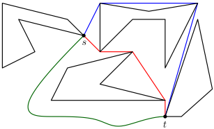
In all these cases, the problem can be abstractly formulated as an ESP instance in the plane by defining obstacles (stationary machines in a production hall, swamps/rocks in a hiking area, islands in the ocean) as polygons and specifying two locations as start/end point, see Figure 1 for an example. Here, three paths from s to t (both obstacle vertices) are depicted with the dotted/red one being the shortest.
It is well known that a shortest path between two obstacle vertices consists solely of edges of the visibility graph, which is a graph on all obstacle vertices with edges between any two vertices/nodes that are mutually visible. Unfortunately, due to the typically very large number of edges in the visibility graph, its construction and even more the explicit storage for non-miniscule problem instances is rather impractical. For example, in [Funke et al., 2024], the authors report on the sizes of visiblity graphs of instances derived from the coastlines of islands in the Mediterranean sea: there, for an instance with only 316k obstacle vertices, the respective visibility graph had more than half a billion edges.
This motivates the first contribution of this work, the simplification of an ESP instance such that the resulting visibility graph becomes manageable - both with respect to construction time as well as storage. Crucial property of our simplification is that distances in the simplified instance always lower bound the distances in the original instance. Hence, these distances can be used, e.g., to guide an A∗ type algorithm like Polyanya [Cui et al., 2017] or to assess the quality of an approximate solution computed, e.g., as in [Funke et al., 2024].
Yet, even if we manage to simplify an ESP instance such that it can comfortably be stored in main memory, the typically very high density of visibility graphs makes shortest path distance computations in this graph via Dijkstra-like algorithms comparatively slow. A natural solution is to apply speed-up techniques like Contraction Hierarchies, [Geisberger et al., 2012a], which, after some quick preprocessing, can answer shortest path queries within milliseconds or faster even on graphs with millions of nodes. Unfortunately, the high density of visibility graphs often renders the preprocessing phase of these techniques infeasible.
So the second contribution of this work is the efficient construction of a data structure for quickly retrieving shortest path distances in visibility graphs based on the hub labeling approach. Such schemes have been applied extensively to relatively sparse graphs like road networks and lead to query times that are amongst the fastest possible, see [Cohen et al., 2003], [Abraham et al., 2012]. But they are not that widely used in practice due to their considerable space consumption, which is at least one order of magnitude above that of the underlying graph for all applications of hub labeling we have encountered. An efficient technique to quickly estimate the importance of vertices of the visibility graph is crucial for the successful instrumentation of a hub labeling scheme. We propose such a method based on a new notion of node reach and show experimentally that the resulting lookup data structure uses roughly the same space as the visibility graph, yet yields query times that are faster by several orders of magnitude. On top of that we propose a method to efficiently answer one-toall distance queries achieving a speedup of around 30 compared to Dijkstra's algorithm.
1.1 RelatedWork
The visibility graph for an ESP instance with n polygon vertices can be computed in time O(n log n + K) where K denotes the number of edges of the resulting visibility graph, see [Ghosh and Mount, 1991]. Unfortunately, K could be very large - Θ(n2 ) in theory, but also prohibitively large in practice. Another group of algorithms based on the idea of a continuous Dijkstra is able to beat the inherent Ω(n2 ) lower bound of visibility-graph-based approaches. [Mitchell, 1996] achieved a running time of O(n3/2+δ ) for any δ > 0, which later was improved to an optimal O(n log n) in [Hershberger and Suri, 1999]. These algorithms are extremely complex and mostly of theoretical interest. A conceptually simple fully polynomial time approximation scheme (FPTAS) which guarantees a result of cost at most (1 +O(ϵ)) times the optimum in running time O( nϵ log 1ϵ ( 1 √ϵ + log n)) was presented in [Aleksandrov et al., 2000]. It essentially computes a very fine discretization to meet the quality guarantee and then runs Dijkstra on that discretization. The constants involved make this approach unsuitable in practice, even for small problem instances. More on the practical side, Polyanya [Cui et al., 2017] carefully instantiates A∗ on a navigation mesh and hence does not require any precomputation (apart from an underlying navigation mesh). It computes the optimal shortest path and has been shown to outperform other state-of-the-art algorithms. For dynamic settings, where even the precomputation of a navigation mesh is not feasible, [Hechenberger et al., 2020] allows for efficient queries, though considerably slower than e.g. [Cui et al., 2017]. Finally, in last year's IJCAI, [Funke et al., 2024] present a data structure that after modest preprocessing can answer approximate shortest path queries for instances with several million obstacle vertices in the milliseconds range. On average their returned paths were less than 2% longer than the optimal paths. Instance-based guarantees on the quality of the resulting paths were obtained via lower bounds without specifying the computation time.
Note that in dimensions 3 and up, computing shortest paths amidst polyhedral obstacles becomes NP-hard [Canny and Reif, 1987]. Here lower bounds become even more important, as computing an exact solution is usually not a viable option. We only consider the planar case in this paper, though.
2 Preliminaries
In the following we give a brief recap of the hub labeling scheme from [Cohen et al., 2003] and [Abraham et al., 2012] as they are the basis for our approach presented in Section 4.
2.1 Shortest Path Distances via Hub Labeling
We consider the shortest path problem in visibility graphs G(V,E) with |V | = n, |E| = m where each vertex v ∈ V has an associated point location in the Euclidean plane. The length of an edge e = {v, w} ∈ E is set to be the Euclidean distance between the points associated with v and w respectively. The length of a path π in G is the sum of its edge lengths. For a point-to-point query, we are given a source s ∈ V and a target t ∈ V and want to find the length d(s, t) of the shortest path from s to t in G. The standard solution is Dijkstra's algorithm [Dijkstra, 1959] which can compute distances to all nodes from a source node in time O(m+n log n).
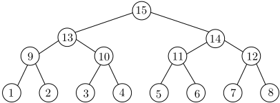
In many applications where many queries have to be answered, Dijkstra's algorithm is too slow. There are labeling algorithms like [Cohen et al., 2003] which preprocess the graph and create a label L(v) for each vertex v such that the distance between given nodes s, t ∈ V can be computed just by inspecting L(s) and L(t). For our work, we consider the special case of hub labeling where the label L(v) consists of a sequence of pairs (u, d(v, u)); the vertex u is a so-called hub for v. The created labels must obey the cover property: for any two vertices s, t ∈ V , L(s) ∩ L(t) must contain at least one vertex on the shortest s-t-path as a hub. To answer a query, one can simply inspect all vertices u ∈ L(s) ∩ L(t), pick the one minimizing d(s, u)+d(t, u), and return the sum. If each label is sorted by the hub vertex IDs, this can be done by a sweep in time O(|L(s)| + |L(t)|). In our example from Figure 4, we have L(2) = {(2, 0), (9, 1), (13, 2), (15, 3)} and L(11) = {(11, 0), (14, 1), (15, 2)}. So the shortest path distance of 5 between node 2 and 11 is determined by hub 15, which is present in both labels. For a hub labeling to be efficient we obviously prefer short labels.
A popular variant of hub labeling are so-called canonical labelings. They are based on a total order ϕ on the vertices. The label L(v) consists of all the vertices that are the highest rank vertex for a shortest path from v to some w. Canonical labelings were shown to satisfy the cover property, see [Abraham et al., 2012]. The most popular technique in practice to find a good total order ϕ is as a by-product of another speed-up technique called contraction hierarchies (CH). In fact, once a CH is available, the respective canonical labeling can be found very efficiently. We briefly recap CH in the following subsection.
Hub Labeling schemes are known for extremely fast query times, but at the cost of a quite considerable space consumption, which is typically at least one magnitude above the space required to store the graph itself, see [Abraham et al., 2012] for results on several (sparse) graph classes. In practice people often stick with slower query times, e.g., achievable via CH. Note that to our knowledge, only very sparse graphs have been considered so far for the use of hub labeling schemes.
2.2 Hub Labeling via Contraction Hierarchies
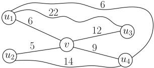
Contraction Hierarchies (CH) [Geisberger et al., 2012a] are one of the most popular acceleration techniques for shortest path queries due to their low space consumption and yet decent speedup. In their preprocessing phase, nodes are contracted one by one in a certain order, see Figure 2 for an example. The resulting shortcuts and the order in which the contraction took place are the result of the preprocessing phase and allow subsequent source-target queries to be answered about four orders of magnitude faster than Dijkstra.
There is a very simple and efficient way of computing a hub labeling (HL) based on a precomputed CH, allowing for even faster source-target distance queries. Essentially, the label of a node consists of all nodes visited during a CH query from a node with their respective distances. Pruning nodes with suboptimal distances from labels, this allows for distance queries within few microseconds even on continent-sized graphs, see [Abraham et al., 2012].
In [Bast et al., 2016] a road network of Western Europe was considered with about 18 million nodes and 42.5 million edges. The CH preprocessing took a mere 5 minutes and resulted in less than 40 million shortcut edges. After that, a source-target query could be answered within 110µs, which is more than 104 times faster than the average Dijkstra query time of 2.2 seconds. Based on the CH, a HL could be constructed within about 37 minutes which then allowed for source-target distance queries within 0.56µs. Yet, the space consumption of the constructed HL is quite enormous with an average of 90 hubs per label. While the original graph together with the CH took less than 1 GB of memory, the HL required about 18GB. In practice, CH query times often suffice, so many real-world routing systems are not HL-based.
3 Shrunk Graph Creation
The basic idea of our simplification routine is quite simple: given an ESP instance with a set of obstacle polygons, we replace each single obstacle polygon P by a simpler (i.e., fewer vertices) polygon P ′ with P ′ ⊆ P . The latter guarantees that distances between any two points in the original instance are lower bounded by the distances in the simplified instance. As P ′ could be viewed as a shrunken version of P we will call the algorithm described in the following Shrinker.
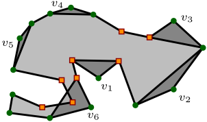
Note that this is different from another popular technique where each polygon is 'simplified' by its convex hull polygon which typically has fewer vertices but contains the original polygon. Only if the convex hulls of the obstacle polygons are pairwise disjoint can we guarantee that shortest paths only turn at corners of the convex hulls, hence allowing for considerably sparser visibility graphs. As we do not want to rule out instances containing obstacles with intersecting convex hulls, though, we will stick to our original idea of simplification. Our shrinking process repeatedly cuts off convex corners of polygons such that the area of the resulting polygons is a proper subset of the original area, yet as large as possible. Figure 3 shows the principle of our approach.
The basis of our algorithm is a constrained Delaunay triangulation [Chew, 1989] of each polygon. We maintain a priority queue in which all convex corners of the current obstacle polygon simplification are maintained. Their priority is given by the triangular area that would be cut off with them. We then repeatedly cut off the minimum priority corner until a specified fraction of corners has been cut off. In Figure 3 we would cut off the corners v4 and v5 before v3.
Before we cut off a corner v we must ensure that the area we would cut off is contained entirely in the polygon. This check is implemented by traversing the polygon triangulation along the segment connecting the neighbors of v. This segment would form the new polygon boundary, so it needs to lie entirely within the existing polygon. If this segment intersects any polygon boundaries, like it is the case for the corner at v6 in Figure 3, the corresponding corner cannot be cut off. If we cut off a corner we also reconsider their neighbors and update their priorities if necessary. Note that this allows vertices that were non-convex in the original obstacle polygon to become convex later on, and then be cut off.
Observe that we do not need to update the polygon triangulation itself during this process. We only remove convex vertices, so whenever such a segment intersects a boundary edge of the shrunken polygon, it must also intersect a boundary edge of the original polygon, and vice-versa.
In the following we describe various instantiations of our shrinking algorithm.
Individual Polygon Shrinking In this first version we look at each polygon individually and shrink them independently of each other. We can do this by executing the shrinking routine separately for each polygon. This lets us specify different shrinking thresholds for different polygons - absolute or relative. This is the approach used in [Funke et al., 2024] to obtain instance-based quality guarantees for their approximate shortest path computations.
Global Shrinking Shrinking polygons independently of each other ignores that some polygons should keep more vertices not because of their original number of vertices but rather because of their shape or location. Specifically, polygon boundaries may not exhibit the same level of detail everywhere, or between different polygons. We could select in each round globally the eligible corner with minimum area amongst all obstacle polygons.
Locking 'Important' Vertices In the approaches outlined so far we only cared about keeping the obstacle polygon areas as large as possible. These goals do not necessarily coincide with keeping as many shortest paths as close as possible to their original length. This is because some vertices are more important to shortest paths than others. For example, in Figure 3, cutting off node v2 might lose less area than cutting off node v1, yet, v1 can only appear on shortest paths in a very local neighborhood, whereas v2 might appear in global shortest paths between very far locations. So a natural idea is to identify such 'important' vertices which potentially appear in many shortest paths. To that end we compute many shortest paths between random pairs of points and count how many times each vertex is used in a shortest path to obtain an importance ranking. Calculating exact shortest paths, e.g. via Polyanya [Cui et al., 2017], is too expensive for this purpose, so we use approximate shortest paths as constructed by the approach of [Funke et al., 2024], which suffices because they mostly follow the same patterns as the exact ones and can be computed within milliseconds.
4 Hub Labeling on Visibility Graphs
Sparseness is one of the most important characteristics of road networks, which is not surprising due to their nearplanarity. The average degree in a typical road network is less than 6 as Euler's polyhedron formula implies. This is one important aspect that makes CH precomputation efficient, since during the course of the preprocessing phase, for each node, every pair of neighboring nodes (according to original edges as well as shortcuts) has to be considered, see [Geisberger et al., 2012b] and our example in Figure 2. Visibility graphs have a much higher average node degree. While it is easy to construct worst case examples where n node visibility graphs have an average node degree of Θ(n), even real-world visibility graphs exhibit very high node degree. For example, the visibility graph 20kCoast from our experimental section with n = 20,000 nodes has an average degree of 635.8. Summing up over all nodes, more than 7 billion shortcut decisions would have to be made if the ordinary CH construction scheme was employed. Each decision requires some additional effort like a Dijkstra run, albeit quite local.
Hence the popular technique of creating a hub labeling via a previously constructed CH seems not feasible for visibility graphs at all due to their high density compared to road networks, which CH and HL are most frequently used for. Note that in the absence of collinear points, for any edge {u, v} in the visibility graph, u must be a hub for v or vice versa. Hence |E|/|V | is a lower bound on the average hub label size.
4.1 An Alternative HL Construction Strategy
Fortunately, there is a somewhat naive strategy of computing a HL for a graph which does not require the precomputation of a CH beforehand, which relies on the original definition of a canonical labeling. We consider a bijective function ϕ : V → {0, . . . , n-1} on the vertices representing an order on V . The function ϕ is also called a level function. We focus on two nodes v, w ∈ V and want to characterize when w appears in the label of v. Let π = vv0v1 . . . vkw be the shortest path from v to w. According to the definition of canonical labeling, w appears in the label of v if and only if ϕ(w) > ϕ(vi) for i = 0, . . . , k and ϕ(w) > ϕ(v), that is, ϕ(w) is the largest ϕ-value among the nodes in π. So given ϕ, we can naively compute the hub label for a node v by computing a shortest path tree for v, and on all shortest paths from v remembering the distances to nodes with maximum ϕ value, which can easily be done in O(n) time for a given shortest path tree.
An obvious advantage of this approach is that it can be parallelized trivially. Still, the construction time will essentially need to run n full Dijkstras which limits this approach to medium sized graphs. Another problem is to determine a suitable contraction order ϕ. In most CH/HL constructions the contraction order ϕ is determined 'on the fly' while performing the contractions (e.g., by contracting the node with minimum edge difference next, see [Geisberger et al., 2012a]). As argued above, we cannot afford to perform the standard CH construction, so we have to come up with other means for determining ϕ. The approaches proposed in [Abraham et al., 2012] have the severe drawback of requiring Θ(n2 ) space, so they do not apply for all but very small instances. In our experimental section we will see that straightforward strategies like random (choose a random permutation) or based on the degree do not perform favourable.
Reach-based Level Functions
Our idea to quickly compute good level functions ϕ is inspired by the notion of reach as proposed in [Gutman, 2004]. The author defined a very intuitive notion of importance for edges in the graph based on whether they appear in the middle of long (with respect to the cost function) shortest paths. Using that notion, it is possible to prune Dijkstra searches and achieve moderate speedups compared to Dijkstra of around one order of magnitude.
For our purpose, we introduce a hop-based notion of node reach and instrument that for good level functions ϕ resulting in small average label sizes. Again consider a shortest path π = v0v1v2 . . . vi . . . vk and define the reach r(vi, π) of vi with respect to π as min(i, k - i). For a set of of paths Π which all contain node v we set r(v, Π) := maxπ∈Π r(v, π). Intuitively, r(v,Π) is large if v appears 'in the middle' of a long shortest path in Π. As [Gutman, 2004] we interpret a large reach as an indicator for a node to be 'important'. After computing reach values for a set of paths Π, we order the nodes in increasing reach value and assign levels according to their rank in this ordering. In practice, we pick a set of random nodes, compute shortest path trees from each of them and then consider all root-to-leaf paths in the shortest path trees to update the reach values of all nodes. This can be done easily in O(n) time for a given shortest path tree. In our experimental evaluation we will see that even a very moderate number of shortest path trees suffice to obtain level functions ϕ for which the average size of the labels is close to the degree in the original visibility graph.
4.2 One-to-All Queries via Hub-Label-Scan (HLS)
CH and HL were originally intended to speed up sourcetarget queries. Later CH were also instrumented to perform faster one-to-all queries in a method called PHAST [Delling et al., 2013] by performing a normal CH search from the source followed by a scan over all edges towards lower-level nodes in decreasing level-order. With a suitable layout and ordering of the nodes in memory, a speedup of almost a factor of 20 compared to plain Dijkstra could be achieved. If several one-to-all queries have to be performed, further speedup was achieved via parallelization on GPU hardware, which is not the focus of this paper, though. The main reason for the speedup was the increased locality of memory accesses by the scan over all edges compared to the rather chaotic memory accesses of Dijkstra's algorithm.
To instrument HL for quick one-to-all queries one could interpret each hub-distance pair (w, d(v,w)) of a node v as an edge (w, v) with weight d(v,w). In a query from s we first set distances of all nodes in the label of s, and afterwards scan over all edges, setting distances accordingly (note that in this case we do not even have to process the edges in a certain order to guarantee correctness). In our experiments we call this HL-PHAST; unfortunately this approach only led to very moderate speedup compared to Dijkstra (less than a factor of 2). The main reason being that too many unnecessary edges are looked at. See Figure 4 for a simple example.
As a remedy we precompute for each node v the set L-1 (v) of all nodes that contain v in their label (together with their distance). Then our strategy is first to set the distances of all nodes in L(v) and then use L-1 (w) for each w ∈ L(v) to determine the distances to all other nodes. We call this approach Hub-Label-Scan (HLS); in our experiments we observed that HLS yields a speedup of up to a factor of 30 compared to plain Dijkstra. In terms of space consumption, this essentially doubles the space required to store the hub labeling.
5 Experiments
All our algorithms were implemented in C++, compiled with g++ 11.4.0, and executed on a Ryzen 7950x 16-core Desktop machine with 128GB of RAM running Ubuntu Linux 22.04. For geometric computations we used the CGAL library [The CGAL Project, 2023], in particular its geometry kernel, the exact geometric predicates, as well as the constrained Delaunay triangulation code. Unless stated otherwise, averages and maxima were calculated over 1000 trials. Source code and data sets are available on a companion page [Funke, 2024].
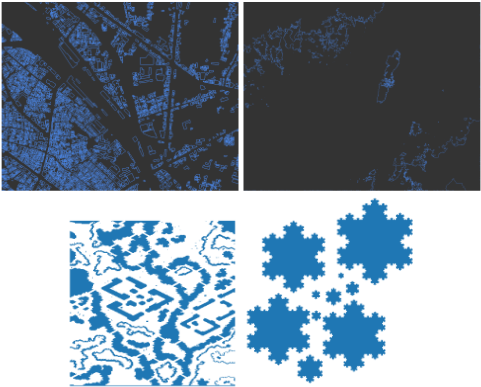
We used several benchmark sets, some derived from game maps from the repository of [Sturtevant, 2012], an urban environment with building footprints extracted from the OpenStreetMap project [The OpenStreetMap Project, 2024], the world's coastlines as also used in [Funke et al., 2024] as well as an arrangement of several Koch snowflakes [Koch, 1904], see Figure 5 for visual depictions of our data sets.
5.1 Shrinking of ESP Instances
To evaluate the lower bound qualities of our shrunken ESP instances, we chose 1,000 random source-target pairs of the original ESP instance and for each of them computed their shortest path using Polyanya [Cui et al., 2017]. If for a given source-target pair dorg, dshrunk are the distance in the original ESP instance and the shrunken instance, we calculated error = 1 - dshrunk dorg as a measure for the quality of the lower bound. Clearly, the smaller the error, the better; error = 0 means we have a lower bound matching the actual distance.
| 0% locked | 2% locked | |||
|---|---|---|---|---|
| avg | max | avg | max | |
| 0.005 · |V | | 0.083% | 1.038% | 0.042% | 0.520% |
| 0.02 · |V | | 0.017% | 0.305% | 0.007% | 0.279% |
| 0.08 · |V | | 0.002% | 0.047% | 0.001% | 0.041% |
| 0.013 · |V | | 0.421% | 6.698% | - | - |
| 0% locked | 2% locked | |||
|---|---|---|---|---|
| avg | max | avg | max | |
| 0.005 · |V | | 0.470% | 9.266% | 0.553% | 9.266% |
| 0.02 · |V | | 0.141% | 3.852% | 0.082% | 2.603% |
| 0.08 · |V | | 0.03% | 1.242% | 0.019% | 1.242% |
| 0.013 · |V | | 1.510% | 17.219% | - | - |
In a first experiment we looked at the world's coastlines with an instance consisting of 651,063 polygons with 15,318,978 obstacle vertices in total. Clearly, this instance does not allow for the construction of its visibility graph.
We used the global shrinking strategy and removed vertices until the desired cardinality of the vertex set was reached, also varying the share of the locked important vertices, that were prohibited from removal. Polygons with less than 4 vertices were removed altogether. For comparison, we also state the results for the shrinking routine from [Funke et al., 2024] provided by the authors in source code which is essentially the individual polygon shrinking strategy. In Table 1 we see the results for source-target pairs chosen uniformly at random in the free (non-obstacle) space. The table reads as follows: when keeping 1/200th of all vertices, the average error of the lower bound is only 0.083%, the maximum 1.038% when we apply the pure global shrinking strategy. If we lock 2% of the remaining nodes by importance as described in Section 3, the error reduces almost by a factor of 2, both on average as well as the maximum within 1,000 queries. The individual shrinking approach as used in [Funke et al., 2024], shown in the last row of the table, fares considerably worse. Even for a larger remaining vertex set of 0.013 · |V |, both average and maximum error are much higher than for our global shrinking strategy with 0.005 · |V | remaining vertices.
At this point we have to mention that choosing random source-target pairs in the free space is probably not the most interesting experiment to conduct. As the oceans make up for most of the earth's surface, most queries start and end in the middle of the ocean without interacting with too many obstacles. So we repeated the experiment but chose the sourcetarget pairs randomly from the obstacle vertices of the original problem instance. The results can be seen in Table 2. We see errors, both on average but also the maxima, increasing by almost an order of magnitude. Yet, the global shrinking strategy with locking of important vertices still yields excellent results, clearly beating the bounds from [Funke et al., 2024] in the last row of the table.
We did not shrink the game instances, as they were so small that the visibility graph can easily be constructed and stored.
| 0% locked | 2% locked | |||
|---|---|---|---|---|
| avg | max | avg | max | |
| 0.005 · |V | | 0.882% | 4.777% | 0.882% | 4.777% |
| 0.02 · |V | | 0.829% | 4.777% | 0.829% | 4.777% |
| 0.08 · |V | | 0.718% | 4.158% | 0.718% | 4.158% |
| 0.013 · |V | | 0.907% | 4.777% | - | - |
| n | m | avg degree | neighbor pairs | |
|---|---|---|---|---|
| 20kCoast | 20,000 | 12.7 · 106 | 635.8 | > 7 · 109 |
| 40kCoast | 40,000 | 40.6 · 106 | 1016.0 | > 45 · 109 |
| fullCoast | 188,269 | 173 · 106 | 920.9 | > 211 · 109 |
| Labyrinth | 16,354 | 1.39 · 106 | 85.2 | > 84 · 106 |
| Expedition | 21,603 | 2.13 · 106 | 98.6 | > 170 · 106 |
| Cauldron | 32,716 | 2.40 · 106 | 73.3 | > 151 · 106 |
| Flake | 150,528 | 66.9 · 106 | 444.4 | > 53 · 109 |
Finally, in Table 3 we see the results for the urban environment of Tokyo. Here both global shrinking as well as locking of important vertices hardly has any effect. This could be due to the completely different scene characteristics; as most obstacles have very few vertices, it is more about removing some obstacles altogether than simplifying them.
Note that none of the shrinking processes took more than 1 minute, so we refrained from a detailed timing analysis.
5.2 Accelerated Distance Computation
For the evaluation of our speed-up schemes for distance computation in visibility graphs we used the graph instances in Table 4. We have a visibility graph of the world's simplified coastlines with around 188k vertices, and two subgraphs thereof with 20k and 40k vertices, respectively. Additionally we have three game maps from the repository of [Sturtevant, 2012] with sizes of around 16k, 21k and 32k. Most game maps have rather restricted visibility due to the presence of many obstacles, so their visibility graphs are less dense that those of coastline graphs. Finally we have an instance of a Koch flake arrangement with around 150k vertices. As mentioned before, we can easily derive from the node degrees of the visibility graph a lower bound on how many shortcut decisions a CH construction algorithm would have to make to compute the CH. We see that even for the small graph 20kCoast, this number is more than 7 billion, making the standard CH construction impractical since every decision also requires a witness search. The 20kCoast/40kCoast/fullCoast visibility graphs need around 291MB/931MB/4GB in main memory, including additional information like coordinates. So they are easily accommodated within a desktop PC's RAM.
Different Level Functions for HL Construction
We evaluated several strategies for determining the level functions on the smallest coastline graph: random chooses as ϕ a random permutation; degree assigns number 1 to n according to increasing degree of the nodes; reach-i determines the hop-based reach value from a set of shortest path trees with i random sources. In Table 6 we list both construction time for the level function as well as the actual HL construction. Unsurprisingly, the latter is essentially unaffected by the level function; the former scales linearly with the number of random sources. The most relevant quantity is the average label size, though. For example when computing the level function based on 1000 shortest path trees, the level function construction took around 5 seconds and resulted in an average label size of 744. This is considerably better than a random level assignment (3,831) as well as a degree-based assignment (1,558). We also observe that it is not worth spending too much time on constructing a good level function. While the average label size improves drastically from reach-10 to reach-50, there is no improvement after reach-10k, so we will use reach-10k for the following experiments. Note that 743 is not too far away from the lower bound for the average label size given by n and m. So we can store hub labels within space of the same order of magnitude that is required to store the visibility graph itself. The results for the other benchmark graphs showed the same behaviour, making reach-10k a universally good choice for determining the level function.
| HL constr time | avg label size | avg HL time | avg Dijk time | HL-PHAST time | HLS time | full Dijk time | ||
|---|---|---|---|---|---|---|---|---|
| 20kCoast | 51s | 743 | 2.3µs | 18ms | 20ms | 4ms | 37ms | |
| 40kCoast | 712s | 1,107 | 3.1µs | 43ms | 56ms | 10ms | 103ms | |
| fullCoast | 16,240s | 1,282 | 3.0µs | 237ms | 304ms | 14ms | 479ms | |
| Labyrinth | 8.9s | 102 | 0.6µs | 3ms | 3ms | 0.1ms | 5ms | |
| Expedition | 19.7s | 280 | 1.6µs | 5ms | 10ms | 1.0ms | 11ms | |
| Cauldron | 37.4s | 148 | 0.9µs | 7ms | 9ms | 0.4ms | 14ms | |
| Flake | 5,153s | 738 | 2.0µs | 100ms | 150ms | 24ms | 224ms |
| level time | avg label size | HL build time | |
|---|---|---|---|
| random | <1s | 3,831 | 103.0s |
| degree | <1s | 1,558 | 103.4s |
| reach-10 | <1s | 843 | 103.2s |
| reach-50 | <1s | 784 | 103.3s |
| reach-100 | <1s | 766 | 102.7s |
| reach-1k | 5.1s | 744 | 103.8s |
| reach-10k | 51.0s | 743 | 104.1s |
| reach-100k | 521.5s | 743 | 103.6s |
Query Times: Source-Target and One-to-All
Of course, the most interesting quantity to measure is query time. For that we considered all benchmark instances, computed the level function based on reach-10k and constructed hub labels. In Table 5, column avg HL time, we report on the average query times for 100 random source-target distance queries using the constructed hub labels. Column avg Dijk time denotes the respective query times for a source-target Dijkstra on the visibility graph (as e.g., employed in [Funke et al., 2024]). We see for our largest graph fullCoast that average query times decrease from 237ms to 3µs, a speed-up of more than 4 orders of magnitude. The hub labeling exhibits an average label size of 1,282 which allows for a space consumption in the same order of magnitude than the original visibility graph even for the largest instance. The construction time was still below 5 hours on our workstation system. For the other, smaller instances, the speedup is less pronounced but still at least 3 orders of magnitude.
In the next experiment we measured the time to compute one-to-all distances using the HL-PHAST scheme as well as our new improved HLS scheme. Again looking at our largest benchmark instance, we see that while a full one-to-all Dijstra takes about 479ms, the HL-PHAST approach yields only a very moderate improvement to 304ms, but our new HLS strategy computed one-to-all distances on average in 14ms - a speedup of more than a factor of 30. This can be explained by the fact that the number of 'edges' to be considered drops from around 241·106 in HL-PHAST to around 17·106 in HLS (and probably some cache effects). The speedup seems to be higher, the bigger the respective instance is, yet, we almost always observe a speedup of a factor at least 10.
6 Conclusions
Large problem instances for the ESP problem typically do not allow the explicit construction and storage of a visibility graph - the natural structure to answer shortest path queries. The first contribution of our paper is a technique to reduce a given ESP problem instance I to a much smaller instance I ′ such that distances within I ′ are very strong lower bounds for distances within I. In particular, our shrinking technique can be used to reduce I to a size such that explicit construction of the visibility graph of I ′ is possible but still yields lower bounds less than 1% below the real distance on average.
The second contribution of our paper is the speedup of distance queries on a given visibility graph. While hub labeling has been long known to be one of the fastest speedup techniques for shortest path distance queries in sparse graphs, it is not often used in practice due to its space overhead which is typically at least one order of magnitude compared to the storage of the underlying graph. We show that for visibility graphs, the space overhead of hub labeling is negligible - in all our experiments, labels use about the same space as the original visibility graph itself. Based on that we can answer point-to-point distance queries in a visibility graph several orders of magnitude faster than plain Dijkstra. For one-to-all queries we propose a new scheme which beats plain Dijkstra by one order of magnitude.
@inproceedings{ijcai2025p946,
  title     = {Fast and Stronger Lower Bounds for Planar Euclidean Shortest Paths},
  author    = {Funke, Stefan and Koch, Daniel and Proissl, Claudius and Staib, Christian and Weitbrecht, Felix},
  booktitle = {Proceedings of the Thirty-Fourth International Joint Conference on
               Artificial Intelligence, {IJCAI-25}},
  publisher = {International Joint Conferences on Artificial Intelligence Organization},
  editor    = {James Kwok},
  pages     = {8510--8517},
  year      = {2025},
  month     = {8},
  note      = {Main Track},
  doi       = {10.24963/ijcai.2025/946},
  url       = {https://doi.org/10.24963/ijcai.2025/946},
}
TY - CPAPER TI - Fast and Stronger Lower Bounds for Planar Euclidean Shortest Paths AU - Funke, Stefan AU - Koch, Daniel AU - Proissl, Claudius AU - Staib, Christian AU - Weitbrecht, Felix T2 - Proceedings of the Thirty-Fourth International Joint Conference on Artificial Intelligence, IJCAI-25 PB - International Joint Conferences on Artificial Intelligence Organization PY - 2025 SP - 8510 EP - 8517 DO - 10.24963/ijcai.2025/946 UR - https://doi.org/10.24963/ijcai.2025/946 ER -Copied
Machine-readable versions of this paper, for tools and AI agents:





