
Interval Selection with Binary Predictions
Proceedings of the Thirty-Fourth International Joint Conference on Artificial Intelligence. Main Track. Pages 8527-8535.
https://doi.org/10.24963/ijcai.2025/948
Keywords
- Planning and Scheduling: PS: Planning under uncertainty
- Planning and Scheduling: PS: Real-time planning
- Planning and Scheduling: PS: Scheduling
- Planning and Scheduling: PS: Planning with Incomplete Information
Abstract
Following a line of work that takes advantage of vast machine-learned data to enhance online algorithms with (possibly erroneous) information about future inputs, we consider predictions in the context of deterministic algorithms for the problem of selecting a maximum weight independent set of intervals arriving on the real line. We look at two weight functions, unit (constant) weights, and weights proportional to the interval’s length. In the classical online model of irrevocable decisions, no algorithm can achieve constant competitiveness. In this setting, we show that a simple algorithm that is faithful to the predictions is optimal, and achieves an objective value of at least OPT - η, with η being the total error in the predictions, both for unit, and proportional weights.
When revocable acceptances (a form of preemption) are allowed, the optimal deterministic algorithm for unit weights is 2k-competitive, where k is the number of different interval lengths. We give an algorithm with performance OPT − η (and therefore 1-consistent), that is also (2k + 1)-robust. For proportional weights, there is an optimal (2φ + 1)-competitive algorithm, where φ is the golden ratio. We present an algorithm with parameter λ > 1 that is 3λ / (λ - 1) -consistent, and (4λ^2 + 2λ) / (λ - 1)-robust. Although these bounds are not tight, we show that for λ > 3.42 we achieve consistency better than the optimal online guarantee, while maintaining bounded robustness.
We conclude with some experimental results on real-world data that complement our theoretical findings, and show the benefit of prediction algorithms for online interval selection, even in the presence of high error.
- [Almanza et al., 2021] Matteo Almanza, Flavio Chierichetti, Silvio Lattanzi, Alessandro Panconesi, and Giuseppe Re. Online facility location with multiple advice. Advances in neural information processing systems, 34:4661-4673, 2021. [ALP, Accessed 2024 09] https:// algorithms-with-predictions.github.io/, Accessed: 2024- 09. Link
- [Angelopoulos and Kamali, 2023] Spyros Angelopoulos and Shahin Kamali. Contract scheduling with predictions. Journal of Artificial Intelligence Research, 77:395-426, 2023.
- [Angelopoulos et al., 2024] Spyros Angelopoulos, Christoph Dürr, Shendan Jin, Shahin Kamali, and Marc Renault. Online computation with untrusted advice. Journal of Computer and System Sciences, 144:103545, 2024.
- [Antoniadis et al., 2020] Antonios Antoniadis, Themis Gouleakis, Pieter Kleer, and Pavel Kolev. Secretary and online matching problems with machine learned advice. Advances in Neural Information Processing Systems, 33:7933-7944, 2020.
- [Antoniadis et al., 2023a] Antonios Antoniadis, Joan Boyar, Marek Eliás, Lene Monrad Favrholdt, Ruben Hoeksma, Kim S Larsen, Adam Polak, and Bertrand Simon. Paging with succinct predictions. In International Conference on Machine Learning, pages 952-968. PMLR, 2023.
- [Antoniadis et al., 2023b] Antonios Antoniadis, Christian Coester, Marek Eliáš, Adam Polak, and Bertrand Simon. Online metric algorithms with untrusted predictions. ACM transactions on algorithms, 19(2):1-34, 2023.
- [Antoniadis et al., 2024] Antonios Antoniadis, Hajo Broersma, and Yang Meng. Online graph coloring with predictions. In International Symposium on Combinato- rial Optimization, pages 289-302. Springer, 2024.
- [Bachmann et al., 2013] Unnar Th Bachmann, Magnús M Halldórsson, and Hadas Shachnai. Online selection of intervals and t-intervals. Information and Computation, 233:1-11, 2013.
- [Berg et al., 2024] Magnus Berg, Joan Boyar, Lene M Favrholdt, and Kim S Larsen. Complexity classes for on- line problems with and without predictions. arXiv preprint arXiv:2406.18265, 2024.
- [Borodin and El-Yaniv, 1998] A. Borodin and R. El-Yaniv. Online computation and competitive analysis, 1998.
- [Borodin and Karavasilis, 2023] Allan Borodin and Christodoulos Karavasilis. Any-order online interval selection. In International Workshop on Approximation and Online Algorithms, pages 175-189. Springer, 2023. Boyar et al., 2017] Joan Boyar, Lene M Favrholdt, Chris- tian Kudahl, Kim S Larsen, and Jesper W Mikkelsen. On- line algorithms with advice: A survey. ACM Computing Surveys (CSUR), 50(2):1-34, 2017.
- [Boyar et al., 2023] Joan Boyar, Lene M Favrholdt, Shahin Kamali, and Kim S Larsen. Online interval scheduling with predictions. In Algorithms and Data Structures Sym- posium, pages 193-207. Springer, 2023.
- [Elias et al., 2024] Marek Elias, Haim Kaplan, Yishay Man- sour, and Shay Moran. Learning-augmented algorithms with explicit predictors. arXiv preprint arXiv:2403.07413, 2024.
- [Emek et al., 2016] Yuval Emek, Magnús M Halldórsson, and Adi Rosén. Space-constrained interval selection. ACM Transactions on Algorithms (TALG), 12(4):1-32, 2016.
- [Feitelson et al., 2014] Dror G Feitelson, Dan Tsafrir, and David Krakov. Experience with using the parallel work- loads archive. Journal of Parallel and Distributed Com- puting, 74(10):2967-2982, 2014.
- [Gabrel, 1995] Virginie Gabrel. Scheduling jobs within time windows on identical parallel machines: New model and algorithms. European Journal of Operational Research, 83(2):320-329, 1995.
- [Garay et al., 1997] Juan A Garay, Inder S Gopal, Shay Kut- ten, Yishay Mansour, and Moti Yung. Efficient on-line call control algorithms. Journal of Algorithms, 23(1):180-194, 1997.
- [Grigorescu et al., 2024] Elena Grigorescu, Young-San Lin, and Maoyuan Song. A simple learning-augmented algo- rithm for online packing with concave objectives. arXiv preprint arXiv:2406.03574, 2024.
- [Gupta et al., 1979] Gupta, Lee, and Leung. An optimal so- lution for the channel-assignment problem. IEEE Trans- actions on Computers, 100(11):807-810, 1979.
- Nicholas G Hall and Michael J Magazine. Maximizing the value of a space mission. Eu- ropean journal of operational research, 78(2):224-241, 1994.
- [Kleinberg and Tardos, 2006] Jon Kleinberg and Eva Tardos. Algorithm design. Pearson Education India, 2006.
- [Kolen et al., 2007] Antoon WJ Kolen, Jan Karel Lenstra, Christos H Papadimitriou, and Frits CR Spieksma. Inter- val scheduling: A survey. Naval Research Logistics (NRL), 54(5):530-543, 2007.
- [Kovalyov et al., 2007] Mikhail Y Kovalyov, Chi To Ng, and TC Edwin Cheng. Fixed interval scheduling: Models, ap- plications, computational complexity and algorithms. Eu- ropean journal of operational research, 178(2):331-342, 2007.
- [Lipton and Tomkins, 1994] Richard J Lipton and Andrew Tomkins. Online interval scheduling. In SODA, vol- ume 94, pages 302-311, 1994.
- [Lykouris and Vassilvitskii, 2021] Thodoris Lykouris and Sergei Vassilvitskii. Competitive caching with machine learned advice. Journal of the ACM (JACM), 68(4):1-25, 2021.
- [Mitzenmacher and Vassilvitskii, 2020] Michael Mitzen- macher and Sergei Vassilvitskii. Algorithms with predictions. In Tim Roughgarden, editor, Beyond the Worst-Case Analysis of Algorithms, pages 646-662. Cambridge University Press, 2020.
- [Plotkin, 1995] Serge Plotkin. Competitive routing of virtual circuits in atm networks. IEEE Journal on Selected Areas in Communications, 13(6):1128-1136, 1995.
- [Purohit et al., 2018] Manish Purohit, Zoya Svitkina, and Ravi Kumar. Improving online algorithms via ml predic- tions. Advances in Neural Information Processing Sys- tems, 31, 2018.
- [Rohatgi, 2020] Dhruv Rohatgi. Near-optimal bounds for online caching with machine learned advice. In Proceed- ings of the Fourteenth Annual ACM-SIAM Symposium on Discrete Algorithms, pages 1834-1845. SIAM, 2020.
- [Tomkins, 1995] Andrew Tomkins. Lower bounds for two call control problems. Information processing letters, 56(3):173-178, 1995.
- [Woeginger, 1994] Gerhard J Woeginger. On-line scheduling of jobs with fixed start and end times. Theoretical Com- puter Science, 130(1):5-16, 1994.
References were extracted automatically from the PDF and may contain errors.
Full text extracted automatically from the PDF; figures, tables and equations may differ. The PDF is the version of record.
1 Introduction
We consider the problem of online interval selection, or interval scheduling on a single machine, where real-length intervals arrive online, and we must output a set of non- Motivated by advancements in machine learning and access to a plethora of data, there has been an effort to equip online algorithms with possibly erroneous predictions about the input instance. Such algorithms are able to achieve much better performance when these predictions are accurate, overcoming some pessimistic bounds of competitive analysis, and helping to bridge the gap between theory and practice. Various classical online problems such as ski rental and non-clairvoyant job scheduling [Purohit et al., 2018], caching [Lykouris and Vassilvitskii, 2021], facility location
1 An extended version of the paper can be found at: https://arxiv.org/abs/2502.10314
| Unit | Proportional | |
|---|---|---|
| Irrevocable (randomized) | Ω(n) [2013] | Ω(log∆) [1994] |
| Revocable (deterministic) | 2k∗ [2023] | (2ϕ+1)∗ [1997] |
[Almanza et al., 2021], metrical task systems [Antoniadis et al., 2023b], and matching [Antoniadis et al., 2020] have been considered in this model. See [Mitzenmacher and Vassilvitskii, 2020] for a more detailed survey on the topic, and ALP for an online repository of relevant papers. Predictions are also a form of untrusted advice [Angelopoulos et al., 2024], a natural extension of the model of online algorithms with advice [Boyar et al., 2017] when the advice is imperfect. Advice research tends to be more information theoretic, focusing on tradeoffs between the number of advice bits and the quality of the solution. Although predictions are often available as offline information, given to the algorithm in advance, we consider a model where a prediction is associated with each input item, and is also given online. This is quite natural and has been considered before for problems such as paging, graph coloring, and packing ([Lykouris and Vassilvitskii, 2021; Rohatgi, 2020; Antoniadis et al., 2023a; Antoniadis et al., 2024; Grigorescu et al., 2024]). This setting also allows for an oracle to adapt as more of the input is revealed, enabling research where there are different bounds on the quality of later predictions, and allowing one to tailor the predictor algorithm directly [Elias et al., 2024]. Furthermore, we use binary predictions, which has our model falling in line with work considering limited size, or succinct predictions [Antoniadis et al., 2023a; Berg et al., 2024; Angelopoulos and Kamali, 2023].
Related work. Table 1 shows the most relevant existing work in the conventional online setting. In the case of irrevocable decisions, no algorithm (even randomized) can achieve a constant competitive ratio. For the relaxed model of revocable acceptances, we use an asterisk to indicate that the competitive ratio is optimal. In the context of randomized algorithms and revocable acceptances, [Emek et al., 2016] give a 6-competitive algorithm for unit weights, while we know of no work improving upon the (2ϕ + 1)-competitive algorithm.
[Boyar et al., 2023] is the most closely related work to our problem with predictions, and motivated our study. They consider the case of unit weighted intervals on a line graph, and give an optimal deterministic algorithm in the setting of irrevocable decisions with performance OPT - η for a different set of predictions and error measure. We extend their work using (possibly adaptive) predictions of limited size, considering an additional weight function of interest, and initiating the study of these problems with revocable decisions.
Structure of the paper. In section 2 we formally define the model, including our predictions and error measure. Section 3 is about the model of irrevocable decisions, whereas in section 4 we allow for revocable acceptances. We conclude with some experiments on real-world data (section 5) that showcase the usefulness of our predictions, and complement our theoretical results.
2 Problem Setting, Definitions and Discussion
In the problem of interval selection, an instance consists of a set of intervals arriving on the real line. Each interval is specified by a starting point si and an end point fi, with si < fi, and it occupies space [si, fi). The conventional notions of intersection, disjointness, and containment apply. Two intervals can conflict because of a partial conflict, or because of proper inclusion. In the latter case, we say that the smaller (larger) interval is subsumed (subsumes) by the other. Each interval I is also associated with a weight w(I). The goal is to output a set of disjoint intervals of maximum weight. We focus on two types of weight functions, unit weights where w(I) = 1 for all I, and proportional weights where w(I) = fi-si. With unit weights, we want to accept as many intervals as possible, whereas with proportional weights, we want to cover as much of the line as possible.
The sequence of the intervals arriving online is chosen by an adversary with full knowledge of the algorithm. In the conventional model of irrevocable decisions, each accepted interval is final and will be part of the final solution. A well studied relaxation of the model is allowing for revocable acceptances, where any new interval may be accepted by displacing any conflicting intervals in the solution, but every rejection is final. This is sometimes also referred to as preemption.
We measure the performance of an online algorithm using worst case competitive analysis [Borodin and El-Yaniv, 1998]. Let ALG denote the total weight of the algorithm's solution, and OPT be the total weight of an optimal solution. An algorithm is strictly c-competitive, if for all instances and input permutations, we have that OPT ALG ≥ c. We also refer to ALG as the performance of the algorithm. Lastly, we will use ALG (respectively OPT) to denote the set of intervals in the algorithm's (optimal) solution. The meaning should always be clear from context.
Predictions. Every interval is associated with a binary prediction that becomes known at the time of the interval's arrival, denoting whether or not that interval is part of some fixed optimal solution. More precisely, Prd(I) = 1 means interval I is predicted to be optimal, and Prd(I) = 0 means that it is predicted to not be optimal. Let I denote the set of all intervals in the instance. We define -→p = (Prd(I1), Prd(I2), ..., Prd(I|I|)) to be the binary vector of all the online predictions. Let also -→ p+ be the predictions vector when all predictions are accurate, and -→ p- = -→ p+.
Error. Every inaccurate prediction introduces an amount of error. Let η(I) be the amount of error introduced by interval I. If the prediction of I was accurate, we define η(I) = 0. If I was wrongly predicted to be non-optimal, let η(I) = w(I), and if I was wrongly predicted to be optimal, and C is the set of optimal intervals I conflicts with, let η(I) = ∑J∈C w(J) - w(I). Let the total error be η = ∑I∈I η(I). One may fix any optimal solution to measure the error against. We use ηmax to denote the maximum possible error, i.e. ηmax = η when -→p = -→ p-.
A common approach to evaluate algorithms that use predictions is to focus on an algorithm's consistency and robustness. We say that an algorithm is γ-consistent if it is γ-competitive, whenever the predictions are accurate, i.e. -→p = -→ p+. We say that an algorithm is ζ-robust, if it is ζ-competitive regardless of the accuracy of the predictions. There is usually a trade-off between consistency and robustness, and the goal is to design algorithms with consistency close to 1, and robustness that is not far worse than the competitiveness of the best predictionless, online algorithm.
Most of our proofs work by using a charging argument, where we map the weight of optimal intervals to the weight of intervals taken by the algorithm, and sometimes error. This charging is usually defined in an online manner, and throughout the execution of the algorithm, we use Φ(I) to refer to the total amount of charge to interval I. In the model of revocable acceptances, we will distinguish between direct, and transfer charging. Transfer charging (TC) occurs at the moment a new interval is accepted by replacing existing intervals, and refers to the amount of charge it inherits because of this. Direct charge (DC) takes place afterwards, whenever an interval causes optimal intervals to be rejected. We use TC(I) (respectively DC(I)) to denote the amount of transfer (direct) charge of an interval, with Φ(I) = TC(I) + DC(I).
We also use the notion of a predecessor trace, which is analogous to Woeginger's predecessor chain [1994] in the real-time model. If I is an interval in the algorithm's solution, the predecessor trace P of I is the maximal list of intervals (P1, P2, .., Pk = I), such that Pi was at some point accepted by the algorithm, but was later replaced by Pi+1.
3 Irrevocable Acceptances
In utilizing access to predictions, a natural algorithm to first consider is one that simply follows the predictions. We therefore present algorithm 1, which is the main subject of this section.
Algorithm 1 Naive
Is ← Set of intervals currently in the solution conflicting
if Prd(I) = 1 and Is = ∅ then
On the arrival of I: with I Take IUnit weights. We first consider the case of unit weights, and prove the following (positive) result on the performance of algorithm Naive.
Theorem 3.1. Algorithm Naive achieves ALG ≥ OPT - η for interval selection with unit weights.
Proof. The proof works by mapping optimal intervals to error, and to intervals taken by the algorithm, given that every missed optimal interval can be associated with at least one unit of error. Let OPT be an optimal solution, and let ALG be the algorithm's solution. For each unit of error, we define an error element h. Let H = {h1, ..., hη} be the set of error elements. Let HI ⊆ H, be the set of error elements corresponding to the error η(I). It holds that HI ∩HJ = ∅ for any two distinct intervals I, J, and ⋃I HI = H.
We define an injective mapping F : OPT → ALG ∪ H as follows: Let Iopt be an optimal interval. If Iopt is taken by the algorithm, it is mapped onto itself. If Iopt is not taken by the algorithm, there are two possibilities. The first possibility is that Prd(Iopt) = 1, but Iopt conflicted with another interval Ic taken by the algorithm. For Ic to have been taken, it means that Prd(Ic) = 1, and |HIc ∪ {Ic}| > 0 because Ic conflicts with Iopt. In this case we map Iopt to an error element hc ∈ HIc , or Ic itself. Even if more optimal intervals were not taken because they conflicted with Ic, there will be enough distinct elements in HIc ∪{Ic} to map them to.
The second possibility is that Iopt was not taken, because Prd(Iopt) = 0. In this case, we have that |HIopt | = 1, and we can map Iopt to the error element of its own prediction. In conclusion, we have that ALG+ |H| ≥ OPT, and we get the desired bound.
Corollary 3.2. Algorithm Naive is 1-consistent.
Theorem 3.3. For every deterministic algorithm, there exist a unit weights instance and predictions, such that ALG = OPT - η.
Proof. Let an interval Ibig arrive first, with Prd(Ibig) = 0. If the algorithm rejects it, no more intervals arrive, and we have ALG = 0, OPT = 1, η = 1. If the algorithm takes Ibig, two non-conflicting intervals arrive next, I1 and I2, both subsumed by Ibig, with Prd(I1) = 0 and Prd(I2) = 1. In this case, we have ALG = 1, OPT = 2, η = η(I1) = 1. In both cases, the equality holds. One can repeat this construction for an asymptotic result.
Corollary 3.4. Algorithm Naive is optimal for unit weights in the model of irrevocable acceptances.
[Boyar et al., 2023] were the first to consider the problem of interval selection with unit weights and irrevocable decisions, and they get the same (syntactically) performance, using a different algorithm, and a different set of predictions and error measure. In comparing our result to theirs, we note that our predictions are information theoretically strictly weaker than theirs 2 , and can in fact easily be extracted from theirs, allowing our algorithms to operate in their model. Furthermore, their predictions-following algorithm is enhanced with a greedy aspect in order to achieve this optimal performance. As we will see in section 5, experimental results on real-world data suggest that for some error ranges, pure greediness is arguably a more important attribute than the use of predictions for getting a good solution, and the combination of both in the context of revocable acceptances works best.
2 Their predictions consist of the entire input instance given in advance.
In the case of proportional weights, algorithm Naive achieves the same performance as in the case of unit weights.
Theorem 3.5. Algorithm Naive achieves ALG ≥ OPT - η for interval selection with proportional weights.
A proof can be found in the full version of the paper.
Theorem 3.6. For every deterministic algorithm, there exist a proportional weights instance and predictions, such that ALG = OPT - η.
Proof. Let I1 arrive first with Prd(I1) = 0. If the algorithm doesn't accept I1, no more intervals arrive, and we have that ALG = 0, OPT = w(I1), and η = w(I1). If the algorithm accepts I1, let two intervals I2 and I3 arrive next, with w(I2) = w(I1), Prd(I2) = 1, w(I3) = 2w(I1) and Prd(I3) = 0. In this case we have ALG = w(I1), OPT = 3w(I1), and η = η(I3) = 2w(I1). In both cases the equality holds. One can repeat this construction for an asymptotic result.
Corollary 3.7. Algorithm Naive is optimal for proportional weights in the model of irrevocable acceptances.
4 Revocable Acceptances
Given the difficulty of the problem(s) in the conventional online model, we now consider the case where acceptances are revocable, but rejections are final, a relaxation of the model that is commonly studied for the problem of interval selection. A new interval can now always be accepted by displacing any intervals in the solution conflicting with it. For unit weights, [Borodin and Karavasilis, 2023] give an optimal algorithm that is 2k-competitive, where k is the number of distinct interval lengths. We will refer to this algorithm as the BK2K algorithm. BK2K is a greedy algorithm, always accepting a new interval when there is no conflict, and whenever a conflict exists, the new interval is accepted only if it is properly included in an interval currently in the solution. We use that as the base logic for our predictions algorithm, and add one more replacement rule, which accepts a new interval I that is only involved in partial conflicts, if Prd(I) = 1. Furthermore, an interval accepted by that rule gets marked, to make sure it cannot be replaced by that rule again. We call this algorithm Revoke-Unit 2. Interestingly, this rule of locally following the predictions once, suffices to give us 1-consistency.
Theorem 4.1. Algorithm 2 achieves ALG ≥ OPT - η.
Due to space constraints, a proof can be found in the full version of the paper. We note that the performance of algorithm 2 on the instance of Theorem 3.3 is exactly equal to OPT - η, and we get the following lemma.
Lemma 4.2. The performance of algorithm 2 cannot be better than OPT - η.
Algorithm 2 Revoke-Unit
M ← ∅ ▷ Set of marked intervals S ← ∅ ▷ Solution set On the arrival of I: Is ← Set of intervals in the solution conflicting with I if Is = ∅ or (Is = {I ′ } and I ⊂ I ′ ) then if I ′ ∈M then M ← M ∪ {I} S ← S ∪ {I} \ {I ′ } ▷ Take I and discard I ′ else if I is only involved in partial conflicts and Prd(I) = 1 and Is ∩ M = ∅ then S ← S ∪ {I} \ Is ▷ Take I, discard conflicts M ← M ∪ {I}We next show that the robustness of Revoke-Unit nearly matches the optimal online guarantee.
Theorem 4.3. With at most k distinct interval lengths, algorithm 2 is (2k + 1)-robust.
Proof. We use a charging argument, building upon the proof of Theorem 3.2 in [Borodin and Karavasilis, 2023], and show that an interval taken by the algorithm can be charged by at most 2k + 1 optimal intervals. The proof can be found in the full version of the paper.
Corollary 4.4. With at most k distinct interval lengths, and predictions with total error η, Algorithm Revoke-Unit achieves ALG ≥ max{OPT - η, OPT 2k+1 }.
Notice how we can choose not to carry over the mark when proper-inclusion replacement occurs, and get a 3k-robust algorithm. Such an algorithm is prone to follow the prediction more often, and it can outperform Revoke-Unit for some small values of error caused by adversarial predictions.
We now look at the case of proportional weights. In the conventional online setting, [Garay et al., 1997] give a 2ϕ + 1 ≈ 4.236-competitive algorithm, while [Tomkins, 1995] gives a matching lower bound. They call their optimal algorithm LR (for length of route), and we include it here for completeness. Unlike the case of unit weights, we now want to accept intervals that occupy as much of the line as possible. Algorithm LR works greedily by always accepting a new interval with no conflicts, and when there are conflicts, it accepts the new interval if its length is at least ϕ times greater than the largest conflicting interval. More generally, using parameter β ≥ ϕ, we have the following lemma:
Lemma 4.5 ([Garay et al., 1997]). Algorithm LR with parameter β ≥ ϕ is (2β + 1)-competitive for the problem of interval selection with proportional weights.
Instead of using algorithm LR as the base of our predictions algorithm, we consider a slightly modified version, which we refer to as LR′ , and which compares the weight of the new interval to the sum of the weights of the conflicting intervals, instead of looking only at the longest interval. Although we do not know the exact performance of algorithm LR′ in the online model, we conjecture it is also (2ϕ + 1)-competitive.
Algorithm 3 LR
Parameter β = ϕ ▷ optimal value for parameter β On the arrival of I: Is ← Set of intervals in the solution conflicting with I if w(I) > β · max{w(J) : J ∈ Is} then
Accept I and displace conflicts
In trying to utilize predictions in the case of proportional weights, we first make the following observations:
Observation 4.6. 1-consistency is unattainable while maintaining bounded robustness.
Proof. To be 1-consistent, the algorithm must be able to replace an interval with an arbitrarily smaller one that is part of the optimal solution. The adversary could then stop the instance, forcing arbitrarily bad robustness.
Observation 4.7. In order to have bounded robustness, it must be that a new interval that is sufficiently large (or reduces ALG sufficiently much) must be accepted (rejected).
Definition 4.8 (α-increasing). An α-increasing algorithm never accepts a new conflicting interval that is less than α times the longest interval it conflicts with.
Lemma 4.9. An α-increasing algorithm (greedy or nongreedy), cannot be better than (2α + 1)-consistent.
Proof. Let an interval I1 arrive first. Let I2 and I3 be intervals that partially conflict with I1 on either side, and w(I2) = w(I3) = α · w(I1) - ϵ. Let I4 with w(I4) = w(I1) - 2ϵ be an interval that is fully subsumed by I4. This instance is depicted in figure 1. The algorithm will never replace I1, while the optimal solution is made of {I2, I3, I4}.

Algorithm LR is a ϕ-increasing algorithm, while the algorithm by Woeginger [1994] for the real-time model is 2-increasing. Our predictions algorithm 4 Revoke-Proportional is 1-increasing. The algorithm works like LR′ , with one additional replacement rule that accepts a new interval that is predicted to be optimal, even if it is not sufficiently larger than what it conflicts with. More precisely, if a new interval is predicted to be optimal and is at least as big as the sum of the weights of the intervals it conflicts with, and none of the conflicting intervals were predicted to be optimal, it will be accepted through the predictions rule. The algorithm takes a parameter λ > 1, which can be thought of as an indicator of how much the predictions are trusted. As λ increases, the consistency bound improves.
Theorem 4.10. Algorithm Revoke-Proportional is 3λ λ-1 - consistent.
Proof. We consider the optimal solution OPT consistent with the fully accurate predictions. We will show that Algorithm 4 Revoke-Proportional Parameter: λ > 1
On the arrival of I: Is ← Set of intervals in the solution conflicting with I Let wc = ∑J∈Is w(J) ▷Weight of conflicting intervals if w(I) ≥ λ · wc then ▷ Main replacement rule Accept I and displace conflicts Return else if Prd(I) = 1 then ▷ Predictions rule if (w(I) ≥ wc and {J : J ∈ Is and Prd(J) = 1} = ∅) thenAccept I and displace conflicts
throughout the execution of the algorithm, we have that Φ(I) ≤ µ · w(I), for every I in the current solution. In the end, we have that ∑I∈ALG Φ(I) = OPT, giving us the µ-consistency of the algorithm.
As in the proof of Theorem 4.3, we consider the notions of transfer charge (TC), and direct charge (DC). We can express Φ(I) = TC(I) +DC(I). A transfer charge occurs whenever accepting a new interval I replaces intervals currently in the solution. In that case, the total charge of those conflicting intervals is passed on as transfer charge to I. Any additional charge to I after its acceptance is through direct charge, namely rejection of subsequent optimal intervals conflicting with I. We will write DCJ (I) to denote the amount of direct charge from interval J to interval I. Whenever an optimal interval is accepted, we consider its weight being directly charged to itself, and it cannot be directly charged again.
Whenever an optimal interval is rejected upon arrival, we charge its weight to the intervals it conflicts with, with its weight being distributed to all its conflicting intervals, in proportion to their weight. Specifically, let Io be the newly arrived optimal interval that is rejected, and Is denote the set of conflicting intervals. Each interval J ∈ Is is directly charged DCIo (J) = w(Io) w(J) wc ≤ w(Io). Furthermore, for an optimal interval to have been rejected, it must be that even the predictions rule failed, and because the predictions are accurate, it must have failed because w(Io) < wc. Because of this, we get that w(Io) w(J) wc ≤ w(J), and therefore DCIo (J) ≤ min{w(Io),w(J)}. An interval I ∈ ALG can be directly charged by at most three different types of optimal intervals: 1) smaller intervals that are subsumed by it, 2) an optimal interval partially conflicting on the left, and 3) an optimal interval partially conflicting on the right. In the case of smaller optimal intervals subsumed by I, the total amount of direct charge from those intervals can be at most w(I). Given that each of the two possible partially conflicting intervals can directly charge I at most w(I), we conclude that for every I ∈ ALG:
We omitted the case where the rejected optimal interval subsumes I, because in that case DC(I) = w(I) and 1 holds trivially. We now focus on the total amount of charge on any interval I ∈ ALG. Let:
We want to make sure that throughout the execution of the algorithm, Φ(I) ≤ µ · w(I). Before any interval is accepted through replacement, intervals in the solution could have only been directly charged through rejected optimal intervals, and because of (1), and the fact that λ > 1, our desired bound holds. We now consider all the cases of an interval being accepted through replacement.
Case 1: I is an optimal interval and it is accepted through the predictions rule. In this case we have that DC(I) = w(I), and we need to look at TC(I). Let Lc and Rc denote the intervals (if any) that I is partially conflicting with on the left and on the right respectively, and let Mc denote the set of intervals that I subsumes. We know that all of these conflicting intervals are not optimal, and they were accepted through the algorithm's main rule. First, notice that for all J ∈ Mc, DC(J) = 0, and Φ(J) = TC(J) ≤ µλ · w(J). Moreover, Lc and Rc had not yet been directly charged by a partially conflicting optimal interval on one side, and therefore we have that Φ(Lc) ≤ µλ · w(Lc) + 2w(Lc), and similarly Φ(Rc) ≤ µλ · w(Rc) + 2w(Rc).
Putting everything together:
The last inequality being true from the fact that the main predictions rule is satisfied. Given also that DC(I) = w(I), we get that Φ(I) ≤ ( µλ + 2)w(I) + w(I) = ( µλ + 3)w(I). With our choice of µ, we have:
Case 2: I is an optimal interval and it is accepted through the algorithm's main rule. This is similar to case 1, with DC(I) = w(I) and w(I) ≥ λ · wc. The same analysis gives us TC(I) ≤ ( µλ +2) w(I) λ , and because λ > 1, the same bound holds.
Case 3: I is not an optimal interval and it is accepted through the algorithm's main rule. In this case we have that DC(I) ≤ 3w(I), and we get that
In conclusion, we have that throughout the execution of the algorithm, for I ∈ ALG, Φ(I) ≤ 3λ λ-1 w(I), and therefore OP T ALG ≤ 3λ λ-1 .
We see that as λ → ∞, the algorithm's consistency goes to 3. We now look at the robustness of algorithm Revoke-Proportional.
Theorem 4.11. Algorithm Revoke-Proportional is 4λ2+2λ λ-1 - robust.
Proof. The argument is similar to the proof of Theorem 4.10. Both direct, and transfer charging work the same way as before. Let µ = 2λ2+3λ+1 λ-1 , and δ = 2λ + 1. We will show that that for every I ∈ ALG, Φ(I) ≤ (µ + δ) · w(I) = 4λ2+2λ λ-1 w(I).
Notice first that the upper bound on direct charging is not as good as before. More precisely, with Io being a newly arrived optimal interval that will be rejected and Is being its conflicting intervals currently in the solution, we have that for every J ∈ Is, DCIo (J) = w(Io) w(J) wc ≤ λ · w(J). More generally, DCIo (J) ≤ min{w(Io), λ · w(J)}. As before, given the three different possible types of conflicts, we have that:
We can now bound the total amount of charge on every interval in the algorithm's solution, throughout its execution. Before any replacement happens, the bound Φ(I) ≤ (µ + δ) · w(I) holds trivially.
Case 1: Interval I is accepted through the algorithm's main rule. We get that:
Case 2: Interval I is accepted through the algorithm's predictions rule. Notice that in this case, all conflicting intervals must have been accepted through the main rule, and not the predictions rule. Because of this, as we showed in case 1, for every J ∈ Is, it holds that Φ(J) ≤ µ · w(J). This helps us bound the amount of transfer charge to interval I.
To summarize, we have shown that in the worst case, Φ(I) ≤ (µ+ δ) · w(I) for every I ∈ ALG. This concludes the proof.
We note that for λ > 2+√5 √5-1 ≈ 3.42, the consistency of our algorithm is already better than 2ϕ + 1, and 22.15robust. We have shown we can get consistency better than
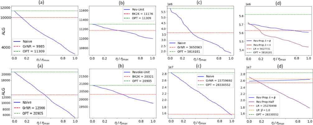
(a) Unit & Irrevocable, (b) Unit & Revoking, (c) Proportional & Irrevocable, (d) Proportional & Revoking
the online bound of LR, while maintaining bounded robustness. We believe further improvement on the bounds of Revoke-Proportional is possible, with an analysis that looks more closely at the dependence between direct and transfer charging.
One may also be able to further improve the algorithm by accepting an interval that is not as big as the sum of its conflicts, making the algorithm a-increasing with a < 1. This would relax the predictions rule further, and make the algorithm more prone to bad choices caused by misleading predictions. In our experiments, we briefly discuss one such algorithm, which we call Revoke-Prop-Half, and which can accept a supposedly optimal interval even if it is half as big as its conflicts.
5 Experimental Results
We use real-world data from scheduling jobs on parallel machines 3 to test our algorithms. More information on the handling of these datasets can be found in a study by [Feitelson et al., 2014]. We focus on two datasets, NASA-iPSC (18,239 jobs) and CTC-SP2 (77,222 jobs). As is usually the case, the performance of algorithms is much better than their worstcase bounds. For every algorithm we average its performance over random permutations of the input instance, for multiple error values. The y axis values for proportional weights are expressed in scientific notation. We note that algorithm GrNR refers to a greedy algorithm without revoking, a very natural algorithm to compare our Naive algorithm against. All other algorithms have been mentioned earlier in the paper. Our experimental results are in line with our intuition, with the predictions algorithms outperforming predictionless algorithms for some values of the error, even when they are not 1-consistent. Especially in the setting of revocable acceptances, even with half of the max possible error, our predictions algorithms perform just as well as their purely online counterparts. In the CTC dataset (figure ??) this is always the case, with the Naive algorithm outperforming GrNR for nearly all values of error. In the case of proportional weights with revoking in figure ??, it is noteworthy that the variant of Revoke-Proportional with λ = 4, outperforms the λ = ϕ variant for some small values of error, but its performance degrades faster. This further validates the notion that the bigger the λ, the more the algorithm follows the predictions.
3 https://www.cs.huji.ac.il/labs/parallel/workload/
We also have to address the seemingly abnormal behavior of algorithm Revoke-Proportional in figure ??(d). As the error increases, so does the performance of Revoke-Proportional, which is counterintuitive and dissimilar to the corresponding plot of figure ??. This is because of the underlying structure of the CTC-SP2 dataset, on which greedy algorithms perform exceptionally well. We showcase this by having included algorithm LR′ with β = 1, the algorithm that accepts a new interval if it is at least as big as everything it conflicts with. As the error increases, a larger number of intervals can be accepted through this clearly beneficial, relaxed predictions rule, which helps explain the improved performance. We also contrast this with algorithm Rev-Prop-Half, which uses a modified predictions rule, that can accept supposedly optimal intervals that are half the weight of their conflicts. This makes the algorithmmore sensitive to the predictions, and its performance falls in line with what we would expect.
In conclusion, algorithms for interval selection can greatly benefit from utilizing imperfect predictions, and remain robust even in the presence of high error.
Acknowledgements
The author would like to thank Allan Borodin, Joan Boyar, and Kim Larsen for many helpful discussions, and for pointing out errors in earlier versions of this work.
@inproceedings{ijcai2025p948,
  title     = {Interval Selection with Binary Predictions},
  author    = {Karavasilis, Christodoulos},
  booktitle = {Proceedings of the Thirty-Fourth International Joint Conference on
               Artificial Intelligence, {IJCAI-25}},
  publisher = {International Joint Conferences on Artificial Intelligence Organization},
  editor    = {James Kwok},
  pages     = {8527--8535},
  year      = {2025},
  month     = {8},
  note      = {Main Track},
  doi       = {10.24963/ijcai.2025/948},
  url       = {https://doi.org/10.24963/ijcai.2025/948},
}
TY - CPAPER TI - Interval Selection with Binary Predictions AU - Karavasilis, Christodoulos T2 - Proceedings of the Thirty-Fourth International Joint Conference on Artificial Intelligence, IJCAI-25 PB - International Joint Conferences on Artificial Intelligence Organization PY - 2025 SP - 8527 EP - 8535 DO - 10.24963/ijcai.2025/948 UR - https://doi.org/10.24963/ijcai.2025/948 ER -Copied
Machine-readable versions of this paper, for tools and AI agents:





