
AccCtr: Accelerating Training-Free Conditional Control For Diffusion Models
Proceedings of the Thirty-Fourth International Joint Conference on Artificial Intelligence. Main Track. Pages 846-854.
https://doi.org/10.24963/ijcai.2025/95
Keywords
- Computer Vision: CV: Efficiency and Optimization
- Computer Vision: CV: Image and video synthesis and generation
Abstract
In current training-free Conditional Diffusion Models (CDM), the sampling process is steered by the gradient, which measures the discrepancy between the guidance and the condition extracted by a pre-trained condition extraction network. These methods necessitate small guidance steps, resulting in longer sampling times.
To address the issue of slow sampling, we introduce AccCtr, a method that simplifies the conditional sampling algorithm by maximizing the sum of two objectives. The local maximum set of one objective is contained within the local maximum set of the other. Leveraging this relationship, we decompose the joint optimization into two parts, alternately maximizing each objective. By analyzing the steps involved in optimizing these objectives, we identify the most time-consuming steps and recommend retraining condition extraction network—a relatively simple task—to reduce its computational cost.
Integrating AccCtr into current CDMs is a seamless task that does not impose a significant computational burden. Extensive testing has demonstrated that AccCtr offers superior sample quality and faster generation times.
- [Bansal et al., 2024] Arpit Bansal, Hong-Min Chu, Avi Schwarzschild, Soumyadip Sengupta, Micah Goldblum, Jonas Geiping, and Tom Goldstein. Universal Guidance for Diffusion Models. In International Conference on Learning Representations, 2024.
- [Chung et al., 2022] Hyungjin Chung, Byeongsu Sim, Do- hoon Ryu, and Jong Chul Ye. Improving Diffusion Models for Inverse Problems using Manifold Constraints. In Ad- vances in Neural Information Processing Systems, 2022.
- [Chung et al., 2023] Hyungjin Chung, Jeongsol Kim, Michael Thompson Mccann, Marc Louis Klasky, and Jong Chul Ye. Diffusion Posterior Sampling for General Noisy Inverse Problems. In International Conference on Learning Representations, 2023.
- [Dhariwal and Nichol, 2021] Prafulla Dhariwal and Alexan- der Nichol. Diffusion Models Beat GANs on Image Syn- thesis. In Advances in Neural Information Processing Sys- tems, 2021.
- [Efron, 2011] Bradley Efron. Tweedie's Formula and Selec- tion Bias. Journal of the American Statistical Association, 2011.
- [He et al., 2024] Yutong He, Naoki Murata, Chieh-Hsin Lai, Yuhta Takida, Toshimitsu Uesaka, Dongjun Kim, Wei- Hsiang Liao, Yuki Mitsufuji, J. Zico Kolter, Ruslan Salakhutdinov, and Stefano Ermon. Manifold Preserving Guided Diffusion. In International Conference on Learn- ing Representations, 2024.
- [Ho and Salimans, 2021] Jonathan Ho and Tim Salimans. Classifier-free diffusion guidance. In NeurIPS Workshop on Deep Generative Models and Downstream Applica- tions, 2021.
- [Ho et al., 2020] Jonathan Ho, Ajay Jain, and Pieter Abbeel. Denoising Diffusion Probabilistic Models. In Advances in Neural Information Processing Systems, 2020.
- [Li et al., 2024] Ming Li, H Kuang T Yang, Z Wang J Wu, and C Chen X Xiao. ControlNet++: Improving Condi- tional Controls with Efficient Consistency Feedback. In European Conference on Computer Vision, 2024.
- [Lin et al., 2014] Tsung-Yi Lin, Michael Maire, Serge Be- longie, James Hays, Pietro Perona, Deva Ramanan, Piotr Dollár, and C Lawrence Zitnick. Microsoft COCO: Com- mon Objects in Context. In European Conference on Com- puter Vision, 2014.
- [Mou et al., 2024] Chong Mou, Xintao Wang, Liangbin Xie, Yanze Wu, Jian Zhang, Zhongang Qi, and Ying Shan. T2I- Adapter: Learning Adapters to Dig Out More Controllable Ability for Text-to-Image Diffusion Models. In AAAI Con- ference on Artificial Intelligence, 2024.
- [Nichol and Dhariwal, 2021] Alexander Quinn Nichol and Prafulla Dhariwal. Improved Denoising Diffusion Prob- abilistic Models. In International Conference on Machine Learning, July 2021.
- [Peng et al., 2024] Bohao Peng, Jian Wang, Yuechen Zhang, Wenbo Li, Ming-Chang Yang, and Jiaya Jia. ControlNeXt: Powerful and efficient control for image and video gener- ation, 2024.
- [Radford et al., 2021] Alec Radford, Jong Wook Kim, Chris Hallacy, Aditya Ramesh, Gabriel Goh, Sandhini Agar- wal, Girish Sastry, Amanda Askell, Pamela Mishkin, Jack Clark, et al. Learning Transferable Visual Models From Natural Language Supervision. In International Confer- ence on Machine Learning, 2021.
- [Rezatofighi et al., 2019] Hamid Rezatofighi, Nathan Tsoi, JunYoung Gwak, Amir Sadeghian, Ian Reid, and Silvio Savarese. Generalized Intersection over Union: A Metric and A Loss for Bounding Box Regression. In Conference on Computer Vision and Pattern Recognition, 2019.
- [Rombach et al., 2022] Robin Rombach, Andreas Blattmann, Dominik Lorenz, Patrick Esser, and Björn Ommer. High-Resolution Image Synthesis With Latent Diffusion Models. In Conference on Computer Vision and Pattern Recognition, 2022.
- [Saharia et al., 2023] Chitwan Saharia, Jonathan Ho, William Chan, Tim Salimans, David J. Fleet, and Mo- hammad Norouzi. Image Super-Resolution via Iterative Refinement. Transactions on Pattern Analysis and Machine Intelligence, 2023.
- [Sara et al., 2019] Umme Sara, Morium Akter, and Moham- mad Shorif Uddin. Image Quality Assessment through FSIM, SSIM, MSE and PSNR: A Comparative Study. Journal of Computer and Communications, 2019.
- [Shen et al., 2025a] Fei Shen, Cong Wang, Junyao Gao, Qin Guo, Jisheng Dang, Jinhui Tang, and Tat-Seng Chua. Long-term talkingface generation via motion-prior condi- tional diffusion model. arXiv preprint arXiv:2502.09533, 2025.
- [Shen et al., 2025b] Fei Shen, Hu Ye, Sibo Liu, Jun Zhang, Cong Wang, Xiao Han, and Yang Wei. Boosting con- sistency in story visualization with rich-contextual condi- tional diffusion models. In Proceedings of the AAAI Con- ference on Artificial Intelligence, 2025.
- [Song and Ermon, 2019] Yang Song and Stefano Ermon. Generative Modeling by Estimating Gradients of the Data Distribution. In Advances in Neural Information Process- ing Systems, 2019.
- [Song et al., 2021] Yang Song, Jascha Sohl-Dickstein, Diederik P. Kingma, Abhishek Kumar, Stefano Ermon, and Ben Poole. Score-Based Generative Modeling through Stochastic Differential Equations. In Interna- tional Conference on Learning Representations, 2021.
- [Song et al., 2023] Jiaming Song, Qinsheng Zhang, Hongxu Yin, Morteza Mardani, Ming-Yu Liu, Jan Kautz, Yongxin Chen, and Arash Vahdat. Loss-Guided Diffusion Mod- els for Plug-and-Play Controllable Generation. In Interna- tional Conference on Machine Learning, 2023.
- [Sun et al., 2024] Yanan Sun, Yanchen Liu, Yinhao Tang, Wenjie Pei, and Kai Chen. AnyControl: Create your art- work with versatile control on text-to-image generation, 2024.
- [Wang et al., 2004] Zhou Wang, Alan C Bovik, Hamid R Sheikh, and Eero P Simoncelli. Image Quality Assess- ment: from Error Visibility to Structural Similarity. Trans- actions on Image Processing, 2004.
- [Yang et al., 2024a] Ling Yang, Zhilong Zhang, Yang Song, Shenda Hong, Runsheng Xu, Yue Zhao, Wentao Zhang, Bin Cui, and Ming-Hsuan Yang. Diffusion Models: A Comprehensive Survey of Methods and Applications. ACM Computing Surveys, 2024.
- [Yang et al., 2024b] Lingxiao Yang, Shutong Ding, Yifan Cai, Jingyi Yu, Jingya Wang, and Ye Shi. Guidance with Spherical Gaussian Constraint for Conditional Diffusion. In International Conference on Machine Learning, 2024.
- [Yu et al., 2023] Jiwen Yu, Yinhuai Wang, Chen Zhao, Bernard Ghanem, and Jian Zhang. FreeDoM: Training- Free Energy-Guided Conditional Diffusion Model. In In- ternational Conference on Computer Vision, 2023.
- [Zhang et al., 2023] Lvmin Zhang, Anyi Rao, and Maneesh Agrawala. Adding Conditional Control to Text-to-Image Diffusion Models. In International Conference on Com- puter Vision, 2023.
- [Zhu et al., 2023] Yuanzhi Zhu, Kai Zhang, Jingyun Liang, Jiezhang Cao, Bihan Wen, Radu Timofte, and Luc Van Gool. Denoising Diffusion Models for Plug-and-Play Im- age Restoration. In Conference on Computer Vision and Pattern Recognition Workshops, 2023.
References were extracted automatically from the PDF and may contain errors.
Full text extracted automatically from the PDF; figures, tables and equations may differ. The PDF is the version of record.
1 Introduction
Recently, diffusion models [Song and Ermon, 2019; Ho et al., 2020; Song et al., 2021] have achieved significant success in generative tasks like generation [Nichol and Dhariwal, 2021; Shen et al., 2025a; Shen et al., 2025b], inpainting [Chung et al., 2023], super-resolution [Saharia et al., 2023]. They employ classifier-guided [Dhariwal and Nichol, 2021] and classifier-free [Ho and Salimans, 2021] techniques for conditional generation. Despite the effectiveness, these methods require additional training. Recent advances addressed these issues by developing training-free methods that leverage the differential loss guidance during the denoising process [Yu et al., 2023; Bansal et al., 2024; Yang et al., 2024b].
Training-free methods avoid extra training but require precise guidance steps for accuracy, increasing sampling time. This is because the tangent space defined by the differential loss can only approximate a local image manifold area. For starting point is remote from target, multiple approximation are needed to span the gap. More denoising iterations are crucial to navigate the curvature of manifold and reach the condition. Current approaches [Chung et al., 2023; Yu et al., 2023; Bansal et al., 2024] use small loss-guided steps to ensure precision, slowing down the process considerably. Yang [2024b] made progress by enabling larger guidance steps through optimization, constraining the steps within boundaries of intermediate data, improving algorithm efficiency.
∗Corresponding author.
Different from Yang [2024b], we improve the efficiency by viewing the sampling process as alternative optimizing two objectives: log p(z0) for unconditional generation and log p(y|z0) for conditional generation, where p(·) denotes the image distribution, p(y|z0) presents the distribution of condition y given image z0 and z0 represents the denoised image of diffusion model at time step 0. We denote the image manifold consisting of z0 asM0. This interpretation streamlines sampling by reducing optimization steps necessary for each objective. Our study reveals that reducing the optimization steps for log p(z0) is straightforward, but not so for log p(y|z0). Taking a well-trained model s(zt), we can estimate the denoised image z0|t, i.e. the projection of zt on the manifold M0, in one step. However, maximizing log p(y|z0|t) involves the gradient of E(y, z0|t,Cψ) and requires multiple gradient descent steps to reach the final outcome.
To reduce the step needed for maximizing the conditional distribution p(y|z0|t), we propose retraining the condition extraction network Cψ(·) to enhance its ability so that the gradient of E(y, z0|t,Cψ) provides a more accurate direction for larger steps. Consequently, we retrain Cψ(·) with two distinct objectives. The first is to ensure that Cψ(z0|t) effectively extracts the necessary conditions from z0|t. The second is to adjust the gradient of E(y, z0|t,Cψ) so that it provides accurate guidance for larger steps.
In summary, our contributions are fourfold: 1. We introduce a novel maximization framework that provides insights into the analysis of training-free CDMs. 2. We identify the key bottleneck in the generation speed of current training-free CDMs using this framework. 3. We propose a loss to retrain the condition extraction network to address this bottleneck. 4. Our model outperforms previous models in efficiency and sample quality.
2 RelatedWork
Conditional Diffusion Models (CDMs) are typically divided into two categories: training-required methods and trainingfree methods. A key aspect of both types of models is the estimation of the conditional score ∇zt log p(zt, y) or its component ∇zt log p(y|zt), which is derived from the relationship ∇zt log p(zt, y) =∇zt log p(zt) +∇zt log p(y|zt).
Training-required CDMs are divided into two main branches. The first branch is the classifier-guided diffusion model [Dhariwal and Nichol, 2021], training a timedependent classifier denoted as pϕ(y|zt, t) to approximate the posterior probability p(y|zt). Consequently, we have ∇zt log p(zt, y) = ∇zt log p(zt) + ∇zt log pϕ(y|zt, t), where the first term represents the unconditional score function, while the second term signifies the adjustment that converts the unconditional score into a conditional one. The other branch is the classifier-free diffusion model [Ho and Salimans, 2021]. This approach employs a neural network to approximate the conditional score ∇zt log p(zt, y). Notable examples include Stable Diffusion [Rombach et al., 2022], ControlNet [Zhang et al., 2023], and ControlNet++ [Li et al., 2024], ControlNeXt [Peng et al., 2024], and AnyControl [Sun et al., 2024]. These models are great at creating realistic images but require more data and training time.
Training-free CDMs eliminates classifier training by defining a loss E(y, z0|t,Cψ) and using its gradient to approximate the conditional score ∇zt log p(y|zt). In the literature, researchers devised various strategies to improve the conditional score estimation. MCG [Chung et al., 2022] addresses deviations with a correction term. DPS [Chung et al., 2023] integrates diffusion sampling with manifold constraints for better noise handling. FreeDoM [Yu et al., 2023] employs a time-travel strategy for robust generation. UGD [Bansal et al., 2024] and DiffPIR [Zhu et al., 2023] guide clean samples z0 to intermediate manifolds zt. LGD [Song et al., 2023] exploits Monte Carlo sampling for estimation refinement. MPGD [He et al., 2024] and DSG [Yang et al., 2024b] apply guidance within data manifolds, with DSG providing a closed-form solution. These approaches often require around 100 sampling steps for quality generation, contrasting with the typically less than 20 steps needed by training-required CDMs.
In this paper, we delve into the rationale behind the increased sampling steps required for training-free CDMs and propose a strategy to enhance their efficiency.
3 Diffusion as Maximization
Diffusion models [Yang et al., 2024a] are understood through different perspectives, such as DDPM [Ho et al., 2020], SMLD [Song and Ermon, 2019], and SDE [Song et al., 2021]. SMLD interprets the diffusion model's role as identifying z0 = argmaxz p(z) that maximizes the image distribution. The projection z0|t of intermediate results zt from the reverse process in DDPM can be viewed as a sequence {z0|T , · · · , z0|1} that progressively maximizes the distribution p(z0|t). This section is dedicated to presenting a maximization view for diffusion model in relation to our method.
3.1 Maximization For Unconditional Diffusion
In this section, we review the sampling process of DDPM. Specifically, diffusion models are represented as: pθ(z0) = ∫ pθ(z0:T ) dz1:T , where z1, . . . , zT are latent variables of the same dimension as the data z0 ∼ q(z0). The joint distribution pθ(z0:T ) is defined by a Markov chain with Gaussian transitions starting from zT ∼ N(zT ; 0, I):
The forward diffusion process, gradually introducing Gaussian noise to the data, is defined by a Markov chain with a predetermined variance schedule β1, . . . , βT :
Let M0 represent the image manifold generated by the diffusion model. This process allows for sampling zt at any step t and deriving its projection ontoM0 in closed form:
Here, ¯ αt := ∏T t=1 αs, αt := 1 - βt. ϵ ∼ N(0, I). ϵ(zt) denote the noised contained in zt and the score function s(zt) := ∇zt log p(zt) satisfying ϵ(zt) = -√1- ¯αts(zt) due to Tweedie's formula [Efron, 2011]. Let ˜µ(zt, z0, t) := √ ¯αt-1βt 1-¯αt z0 + √αt(1-¯αt-1) 1-¯αt zt and ˜ βt := 1-¯αt-1 1-¯αt βt, q(zt-1|zt, z0) can be written as
By defining sθ(zt) as the network to approximate the score function s(zt) and substituting it into Equation (8), we obtain ˆz0|t-1, an estimation for z0 according to zt-1.
We conclude that ˆz0|t is the projection of ˆzt onto the image manifold M0 and the sequence {ˆz0|t} maximizes log p(ˆz0|t). Therefore, we regard the two equations as the solver that maximizes log p(ˆz0|t) on M0.
3.2 Maximization For Conditional Diffusion
Conditional diffusion models employ the conditional score s(zt|y) := ∇zt log p(zt|y) as a substitute for s(zt) in Equation (10), enabling the generation of images conditioned on y. This function is articulated via Bayes' theorem as follows: s(zt|y) = s(zt) +∇zt log p(y|zt). To sidestep training, a practical approach is to use an energy function, defined as: log p(y|zt) = -λE(y, z0|t,Cψ), where z0|t = 1 √ ¯αt (zt + (1 - ¯αt))sθ(zt). In this expression, λ is a positive parameter. Consequently, Equation (10) can be restructured accordingly.
Similar to the discussion for Equation (10) in Section 3.1, the green Equations (11)(12) serve as a solver maximizing the marginal distribution p(ˆz′0|t ). Given Equation (6), we have
Putting this into the yellow Equation (13), we conclude that it operates as a gradient descent step for E(y, ˆz′0|t-1 ,Cψ). Thus, the sequence {ˆz′0|t } maximizes log p(ˆz′0|t ), while the sequence {ˆz0|t} maximizes log p(y|ˆz0|t). To summarize, these equations alternately maximize the two objectives log p(ˆz′0|y ) and log p(y|ˆz0|t) on the image manifold M0 with each step focusing on one objective.
4 Alternative Maximization For Conditional Diffusion
In this section, we frame the conditional diffusion process as an alternating maximization algorithm for two objectives: p(z0|t) and p(y|z0|t). This insight helps us understand why training-free CDMs require more sampling steps and leads to a strategy for speeding up the process.
4.1 The Local Maxima Characteristics
The distribution p(·) is particularly pronounced at the natural image z0. Given that the condition extraction function Cψ(·) is finely tuned for natural imagery, the conditional distribution p(y|z0) := 1C exp (-λE(y, z0,Cψ)) , reaches its zenith when y aligns seamlessly with z0|t. This distribution is more concentrated than p(y|z) for images z in the vicinity of z0, such that p(y|z0) ≥ p(y|z). Thus, for a fixed y, the maximum of p(y|z0) should occur where p(z0) is at its local maximum. This implies that the local maxima of p(y|z), given y, are a subset of the local maxima of p(z). In essence, wherever p(z) experiences a local peak, p(y|z) is also likely to peak, provided that y accurately represents z. This relationship underscores the pivotal role of the conditional distribution in guiding the generative process towards images that not only conform to the natural image distribution but also match the specified conditions.
Algorithm 1 Alternative Maximization Sampling
- 1: Input: The iteration number J, the unconditional diffusion count N for solving p(z0|t) and the conditional correction count M for solving py(z0|t). The time reversal step K.
- 3: ˆzJN ∼N(0, I)
- 4: for j = J, . . . , 1 do
- 5: for n = 0, . . . , N - 1 do
- 6: t ← jN - n
- 8: end for
- 13: end for
- 14: ˆz0|t ← ˆz(M) 0|t
- 15: end for
- 16: Return the result =0
4.2 Alternatve Maximization
We shift focus from the probabilistic details of p(z0|t) and p(y|z0|t) in the following sections, treating them as functions of z0|t under a given condition y. We refer to p(y|z) as py(z), recognizing that the local maxima of py(z) are contained within those of p(z). The conditional generation aims to maximize log p(z0|t, y) by sequentially optimizing log p(z0|t) and log py(z0|t). This strategy, as outlined in the proposition 1, efficiently optimizes the likelihood log p(z0|t, y) = log p(z0|t) + log py(z0|t).
Proposition 1 (Convergence of Alternative Maximization). Let A(z) and B(z) be two functions defined on the same domain. Suppose that: SB, the local maxima point set of B(z), is a subset of SA, the local maxima point set of A(z). Then, the alternating maximization of A(z) and B(z) converges to a local maximum of the function A(z) + B(z).
We provide the proof in the appendix. In light of Proposition 1, the two green Equations (11)(12) in Section 3.2, along with the yellow Equation (13), serve as maximization solvers for log p(z0) and log py(z0). The alternative maximization sampling process is elaborated in Algorithm 1, where the green section and yellow section correspond to the implementation of the green Equations (11)(12) and the yellow Equation (13), respectively. Notably, steps 9, 10, and 11 of Algorithm 1 ensure that the gradient ascent for log py(z0) is consistently performed on the image manifold M0, as characterized by the diffusion model.
5 AccCtr: Accelerating Training-free Conditional Diffusion
The input of Algorithm 1 includes several parameters. In this section, we will examines the impact of the total iterations J, the iterations N for maximizing p(z0|t) (green section), and M for maximizing py(z0|t) (yellow section).
5.1 Why Traning-Free CDMs Sampling Is Slow?
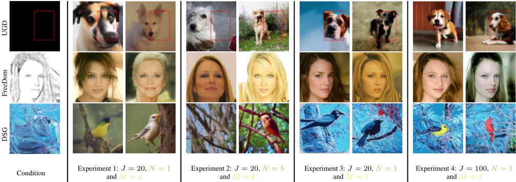
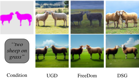
Speeding up the sampling speed requires reducing inference steps. The variation in sampling methods often obscures the root causes of this slowness. Proposition 1 helps break down the sampling process into two phases: maximizing log p(z0|t) via unconditional diffusion implemented by the green Equations (11)(12) and maximizing log py(z0|t) through conditional correction implemented by the yellow Equation (13). By integrating existing algorithms into the framework detailed in the appendix, we can identify the phase that slows down the sampling process. As depicted in Figure 1, we conducted four experiments. The first section outlines the condition y, with each row corresponding to a different CDMs and showing performance under y. Four experiments were tested to ensure consistent behavior across methods.
Experiment 1: With J = 20, N = 1, M = 1, 20 iterations were allocated to maximize both log p(z0|t) and log py(z0|t). Results are in the first section of Figure 1.
Experiment 2: With J = 20, N = 5, M = 1, 100 and 20 iterations maximizes log p(z0|t) and log py(z0|t), respectively. Results are in the second section of Figure 1.
Experiment 3: With J = 20, N = 1, M = 5, 20 iterations were allocated to maximize log p(z0|t) and 100 steps to log py(z0|t). Results are in the third section of Figure 1.
Experiment 4: We set J = 100, N = 1, M = 1, resulting in 100 iterations for both log p(z0|t) and log py(z0|t). Results are in the second section of Figure 1.
Figure 1 shows that the first two experiments lacked control, while the last two succeeded. Thus a higher number of conditional correction iterations J × M is crucial for control; the first two experiments used 20 iterations, while the last two used 100. These results suggest that reducing the optimization steps for log p(z0|t) is tolerable, but cutting steps for log py(z0|t) harms sample quality.
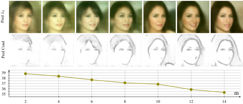
Experiment 5 tracks the development of the extracted condition from the intermediate outputs ˆz(m) 0|t , investigating the impact of reducing maximization steps for log py(z0|t). Figure 2 shows that as m increases, the extracted condition aligns more closely with the target condition. We used MSE loss to measure the difference between the intermediate edge condition and the target edge image. The bottom row of Figure 2 shows a decrease in MSE as m increases, indicating improved guidance conformity across iterations.
These findings suggest that reducing the conditional correction count M can cause a loss of control over the final output, as intermediate conditions may deviate from the target. The issue lies in the linear manifold assumption. The gradient descent approximates the local image manifold using the tangent space. If the starting point is far from the target, additional linear manifolds are needed. Thus, increasing the iteration number for conditional correction is vital for navigating the manifold's curvature and obtaining a sample closer to the target condition.
5.2 Our Approach
Our five experiments suggest that Cψ(·) require more iterations as ∇z0|t E(y, z0|t,Cψ) does not provide accurate estimates for large steps. To reduce the number of maximization steps for log py(z0|t), we propose refining the condition extraction network Cψ(·) to improve its accuracy, enabling more precise gradient directions for larger steps. Therefore, it is logical to retrain Cψ(·) with two distinct objectives.
controllability
(MSE Loss)
The 1st term: L1(y, z0|t,Cψ) is to effectively extract necessary conditions from zt. Here, z0|t represents the projection of zt onto the manifold M0.
The 2st term: L2(y, z0, z0|t,Cψ) is to adjust the gradient of the first term so that it provides accurate directional guidance for larger steps.
The first loss can be constructed using two strategies. The first approach defines L1(y, z0|t, Cψ) = L(y - Cψ(D(z0|t))), where the similarity metric L can be MSE, Cross-Entropy loss, or another appropriate measure depending on the guidance y. D is the pre-trained decoder that converts z0|t into an image, and Cψ is the network for tasks such as segmentation, depth mapping, or HED. A limitation of this method is that it requires different metrics for different guidance types. MSE loss may not always be suitable; for example, cross-entropy loss works better for segmentation guidance. In this paper, we shift the similarity comparison from the pixel domain to the latent domain, as shown in Equation 15, where E is the encoder that converts an image into its latent representation. This approach offers two key benefits: 1) it allows MSE loss for various types of guidance, and 2) it enables high-level latent semantic comparisons [He et al., 2024].
The second loss fine-tunes the gradient for larger time steps, aiming to achieve the final outcome in a single iteration. Putting E(y, z0|t,Cψ) = L1(y, z0|t,Cψ, we employ the conditional score function∇zt log p(zt|y) =∇zt log p(zt)+ ∇zt log py(zt) with∇zt log py(zt) ≈ √ ¯αt∇z0|t log py(z0|t) to replace the score function in Equation 8. This adjustment ensures that the gradient is more accurately aligned for larger steps. Consequently, we obtain:
In this work, we use the two loss terms to retrain the condition extraction network Cψ(·), which is then integrated into Algorithm 1. Given that z0|t can be derived from zt using Equation 8, and zt can be recovered from z0 via Equation 6, we can efficiently train the condition extraction network Cψ(·) with just the pair (y, z0).
6 Experiment
In this section, we conduct thorough experiments and comparisons to showcase the efficacy and strengths of our AccCtr sampling approach.
6.1 Implementation Details
We employed the SD-V1.5 model as the backbone. To facilitate the training process, we selected the Adam optimizer and set its learning rate to 1e-5. With a batch size of 1, the model was subjected to 200, 000 training steps on the COCO2017 dataset [Lin et al., 2014], lasting roughly 60 hours.
| UGD | FreeDom | DSG | Ours | |
|---|---|---|---|---|
| Unconditional Diffusion Count N (Times) | 500 | 100 | 100 | 20 |
| Conditional Correction Counts M (Times) | 3000 | 90 | 90 | 20 |
| Total Sampling Spend (Second) | 2357 | 83 | 53 | 8 |
6.2 Illustrating Sampling Acceleration
In this section, we explore the acceleration capabilities of AccCtr. Proposition 1 suggests that training-free CDMs can be distilled into the optimization of two key objectives. Our experimental results indicate that while the maximum number of iterations for the unconditional objective can be significantly reduced, the same cannot be said for the conditional diffusion, which requires a higher number of iterations. To address this, AccCtr proposes retraining the condition extraction networks Cψ(·) to decrease the number M of conditional correction iterations needed for the conditional objective log py(z0|t).
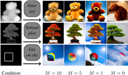
Figure 3 presents the visual quality of images generated by AccCtr for different values of M. It's evident that our method can achieve satisfactory results even at M = 1, potentially greatly enhancing the sampling speed for CDMs. When M = 0, the sampling process does not incorporate conditional control, resulting in outputs that are unaffected by the guidance. Therefore, setting M = 1 represents the quickest scenario for conditional generation. To offer an overview of the acceleration capabilities of our method, we present a quantitative comparison of the running costs in Table 1. We specifically evaluate our method against FreeDoM [Yu et al.,
2023], DSG [Yang et al., 2024b], and UGD [Bansal et al., 2024] with respect to the iteration number N for unconditional diffusion, the iteration number M for conditional correction, and the total sampling time. It can be observed that our method incurs the lowest running costs in Table 1.
6.3 Condition Extraction Network's Compatibility
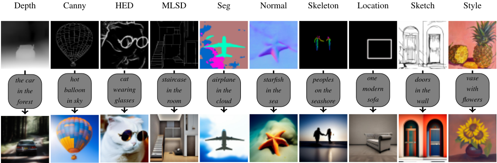
In Section 5.2, we highlighted our condition extraction network assess the similarity between the guidance and intermediate results using MSE. This approach differs from previous methods that employed different metrics for different guidances. Figure 4 shows the visualization results with different guidances, where the similarity is consistently measured by MSE. The results confirm the compatibility of condition extraction networks for diverse guidances.
Replacing existing pre-defined condition extraction networks with ours is viable, as shown in Figure 5 for FreeDoM [Yu et al., 2023], DSG [Yang et al., 2024b], and UGD [Bansal et al., 2024]. The first row shows original results, and the second row shows results with our networks. The sampling quality is comparable, proving our network's compatibility.
| Depth | Canny | Segmentation | HED | |||||||||
|---|---|---|---|---|---|---|---|---|---|---|---|---|
| FID↓ | CLIP↑ | MSE↓ | FID↓ | CLIP↑ | SSIM↑ | FID↓ | CLIP↑ | mIoU↑ | FID↓ | CLIP↑ | SSIM↑ | |
| ControlNet | 19.3954 | 0.2793 | 90.1302 | 17.3429 | 0.2801 | 0.4138 | 22.1217 | 0.2795 | 0.4217 | 20.1402 | 0.2836 | 0.5941 |
| T2I-Adapter | 23.9216 | 0.2913 | 94.9317 | 17.6812 | 0.3011 | 0.3954 | 22.0173 | 0.2995 | 0.2564 | - | - | - |
| ControlNet++ | 18.0139 | 0.2985 | 87.2173 | 20.1487 | 0.3024 | 0.5138 | 24.9371 | 0.2931 | 0.5438 | 16.3124 | 0.3121 | 0.6768 |
| UGD | 26.0034 | 0.2621 | 95.6792 | 26.8452 | 0.2513 | 0.3737 | 27.5437 | 0.2692 | 0.3327 | 28.3487 | 0.2537 | 0.4235 |
| FreeDom | 27.7825 | 0.2579 | 97.1242 | 27.9547 | 0.2487 | 0.3537 | 28.3619 | 0.2465 | 0.3131 | 28.4034 | 0.2472 | 0.4231 |
| DSG | 27.2147 | 0.2466 | 96.5637 | 26.6153 | 0.2571 | 0.3411 | 28.0198 | 0.2538 | 0.3285 | 28.9572 | 0.2514 | 0.4127 |
| Our | 22.4376 | 0.2932 | 86.0179 | 21.3846 | 0.3041 | 0.5217 | 22.9631 | 0.3011 | 0.4018 | 20.6734 | 0.3235 | 0.5104 |
6.4 Ablation Study For Training Loss
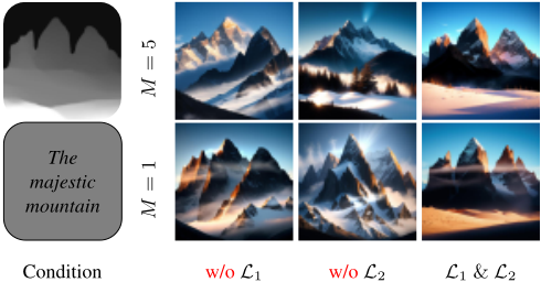
Our training loss for the condition extraction networks Cψ(·) consists of two key terms. In this section, we conduct an ablation study on these terms to assess their individual contributions, with the final results presented in Figure 6. It is clear that without L1, the generation result does not align with the condition, even with a larger number M of conditional corrections. On the other hand, when L2 is removed, controllability remains the same, regardless of the number of conditional corrections. In contrast, using condition extraction networks trained with both terms yields significantly better results.
6.5 Sampling Quality Comparison
In this section, we conduct quantitative comparison for sampling quality comparison. Total six methods including three training-free CMDs (FreeDoM [Yu et al., 2023], DSG [Yang et al., 2024b], UGD [Bansal et al., 2024] ) and three training-required CMDs (ControlNet [Zhang et al., 2023], T2I-Adapter [Mou et al., 2024], ControlNet++ [Li et al., 2024] ) are compared. The test is conducted on COCO2017 validation set with timesteps set to 20. For text alignment, we evaluated the CLIP Scores [Radford et al., 2021]. For conditional consistency, we measured MSE [Sara et al., 2019] for depth maps, SSIM [Wang et al., 2004] for edge maps, and mIoU [Rezatofighi et al., 2019] for segmentation maps. For conditions not originally supported by training-free CDMs, we have integrated our condition extraction network into their existing algorithms. It is evident that AccCtr leads among pioneering training-free approaches in Table 2, and even when compared to training-required methods, our approach remains competitive. For a qualitative comparison, please refer to the supplementary material.
6.6 Balancing Training and Inference Time
Balancing training and inference time is crucial. AccCtrl, compared to training-free methods like FreeDoM [Yu et al., 2023], DSG [Yang et al., 2024b], and UGD [Bansal et al., 2024], markedly decreases inference time but requires additional retraining. Training-required methods including ControlNet [Zhang et al., 2023], T2I-Adapter [Mou et al., 2024], ControlNet++ [Li et al., 2024] generally have faster inference times than their training-free counterparts, but this comes with longer training periods (1000+GPU/hours). However, AccCtrl reduces training time (less than 100GPU/hours) due to its condition extraction network Cψ(·) starting with good initial weights. Thus, without retraining, AccCtrl can still function like traditional training-free methods. In contrast, other training-required methods fail without training. AccCtrl thus offers a favorable trade-off between training and inference time.
7 Conclusion
Slow sampling is a common issue in training-free CDMs. To solve this problem, we introduce a novel framework that reformulates training-free CDMs into the maximization of two objectives. By counting the optimization steps for each objective, we identify the phase that is the bottleneck for sampling speed and propose retraining the condition extraction networks as a strategy to expedite conditional sampling. Our extensive experiments confirm that AccCtr can significantly reduce the computational cost without compromising sample quality. Most importantly, our method exhibits broad compatibility, holding potential to accelerate a variety of other methods. This conclusion underscores the versatility and efficacy of our approach in addressing the common challenge of slow sampling speeds in training-free CDMs.
Acknowledgements
This work was supported by the National Natural Science Foundation of China (62372237, 62332010) and the Major Science and Technology Projects in Jiangsu Province under Grant BG2024042.
@inproceedings{ijcai2025p95,
  title     = {AccCtr: Accelerating Training-Free Conditional Control For Diffusion Models},
  author    = {Dai, Longquan and Wang, He and Zhang, Yiming and Wang, Shaomeng and Tang, Jinhui},
  booktitle = {Proceedings of the Thirty-Fourth International Joint Conference on
               Artificial Intelligence, {IJCAI-25}},
  publisher = {International Joint Conferences on Artificial Intelligence Organization},
  editor    = {James Kwok},
  pages     = {846--854},
  year      = {2025},
  month     = {8},
  note      = {Main Track},
  doi       = {10.24963/ijcai.2025/95},
  url       = {https://doi.org/10.24963/ijcai.2025/95},
}
TY - CPAPER TI - AccCtr: Accelerating Training-Free Conditional Control For Diffusion Models AU - Dai, Longquan AU - Wang, He AU - Zhang, Yiming AU - Wang, Shaomeng AU - Tang, Jinhui T2 - Proceedings of the Thirty-Fourth International Joint Conference on Artificial Intelligence, IJCAI-25 PB - International Joint Conferences on Artificial Intelligence Organization PY - 2025 SP - 846 EP - 854 DO - 10.24963/ijcai.2025/95 UR - https://doi.org/10.24963/ijcai.2025/95 ER -Copied
Machine-readable versions of this paper, for tools and AI agents:





