
Scalable Algorithms for Approximate DNF Model Counting
Proceedings of the Thirty-Fifth International Joint Conference on Artificial Intelligence. Main Track. Pages 2191-2198.
https://doi.org/10.24963/ijcai.2026/244
Keywords
- Uncertainty in AI: Bayesian networks
- Constraint Satisfaction and Optimization: Constraint satisfaction
- Uncertainty in AI: Probabilistic programming
- Uncertainty in AI: Inference
- Constraint Satisfaction and Optimization: Solvers and tools
Abstract
Model counting of Disjunctive Normal Form (DNF) formulas is a critical problem in applications such as probabilistic inference and network reliability.
For example, it is often used for query evaluation in probabilistic databases. Due to the computational intractability of exact DNF counting, there has been a
line of research into a variety of approximation algorithms.
We develop a new Monte Carlo approach with an adaptive stopping rule and short-circuit formula evaluation. We prove it achieves Probably Approximately Correct (PAC) learning bounds and has
asymptotically improved time and randomness complexity compared to previous methods. We also show experimentally that it out-performs prior algorithms by at least three orders of magnitude in running time and scalability.
- [Abboud et al., 2020] Ralph Abboud, İsmail İ Ceylan, and Thomas Lukasiewicz. Learning to reason: Leveraging neural networks for approximate DNF counting. In Proc. of AAAI, 2020.
- [Bacchus et al., 2003] Fahiem Bacchus, Shannon Dalmao, and Toniann Pitassi. Algorithms and complexity results for #SAT and bayesian inference. In Proc. of FOCS, 2003.
- [Bellare and Rogaway, 2004] Mihir Bellare and Phillip Rog- away. Code-based game-playing proofs and the security of triple encryption. Cryptology ePrint, 2004.
- [Borgwardt et al., 2017] Stefan Borgwardt, Ismail Ceylan, and Thomas Lukasiewicz. Ontology-mediated queries for probabilistic databases. In Proc. of AAAI, 2017.
- [Bringmann and Larsen, 2013] Karl Bringmann and Kasper G Larsen. Succinct sampling from discrete distributions. In Proc. of ACM Symposium on Theory of Computing, 2013.
- [Chakraborty et al., 2016] Supratik Chakraborty, Kuldeep S Meel, and Moshe Vardi. Algorithmic improvements in approximate counting for probabilistic inference: From linear to logarithmic SAT calls. In Proc. of IJCAI, 2016. IJCAI
- [Dagum et al., 2000] Paul Dagum, Richard Karp, Michael Luby, and Sheldon Ross. An optimal algorithm for monte carlo estimation. SIAM Journal of Computing, 2000.
- [Dalvi and Suciu, 2007] Nilesh Dalvi and Dan Suciu. Effi- cient query evaluation on probabilistic databases. In Proc. of VDLB, 2007.
- [De Raedt et al., 2007] Luc De Raedt, Angelika Kimmig, and Hannu Toivonen. Problog: A probabilistic prolog and its application in link discovery. In Proc. of IJCAI, 2007. IJCAI
- [Draper and Saad, 2026] Thomas L Draper and Feras A Saad. Efficient online random sampling via randomness recycling. In Proc. of ACM-SIAM Symposium on Discrete Algorithms (SODA), pp 2473-2511, 2026.
- [Dudek et al., 2020] Jeffrey Dudek, Vu Phan, and Moshe Vardi. ADDMC: Weighted model counting with algebraic decision diagrams. In Proc. of AAAI, 2020.
- [Duenas Osorio et al., 2017] Leonardo Duenas Osorio, Kuldeep S Meel, Roger Paredes, and Moshe Vardi. SAT-based connectivity reliability estimation for power transmission grids. Tech Report, 2017.
- [Harris and Srinivasan, 2018] David G Harris and Aravind Srinivasan. Improved bounds and algorithms for graph cuts and network reliability. Random Structures & Algorithms, 2018.
- [Karger and Stein, 1996] David R Karger and Clifford Stein. A new approach to the minimum cut problem. Journal of the ACM, 1996.
- [Karger, 2001] David R Karger. A randomized fully poly- nomial time approximation scheme for the all-terminal network reliability problem. SIAM Review, 2001.
- [Karp and Luby, 1983] Richard Karp and Michael Luby. Monte-carlo algorithms for enumeration and reliability problems. In Proc. of SFCS, 1983.
- [Karp et al., 1989] Richard Karp, Michael Luby, and Neal Madras. Monte-carlo approximation algorithms for enu- meration problems. Algorithms, 1989.
- [Kimmig et al., 2011] Angelika Kimmig, Guy Van den Broeck, and Luc De Raedt. An algebraic prolo for rea- soning about possible worlds. In Proc. of AAAI, 2011.
- [Meel et al., 2017] Kuldeep Meel, Aditya Shrotri, and Moshe Vardi. On hashing-based approaches to approximate DNF- counting. In Proc. of FSTTCS, 2017.
- [Meel et al., 2019] Kuldeep S Meel, Aditya A. Shrotri, and Moshe Y. Vardi. Not all FPRASs are equal: Demystifying FPRASs for DNF-counting. Constraints, 2019.
- [Meel et al., 2021] Kuldeep S Meel, N.V. Vinodchandran, and Sourav Chakraborty. Estimating the size of union of sets in streaming models. In Proc. of PODS, 2021.
- [Narodytska et al., 2019] Nina Narodytska, Aditya Shrotri, Kuldeep S Meel, Alexey Ignatiev, and Joao Marques-Silva. Assessing heuristic machine learning explanations with model counting. In Proc. of SAT, 2019.
- [Naveh et al., 2007] Yehuda Naveh, Michael Rimon, Itai Jaeger, Yoav Katz, Michael Vinov, Eitan Marcu, and Gil Shurek. Constraint-based random stimuli generation for hardware verification. AI Magazine, 2007.
- [Pote et al., 2025] Yash Pote, Kuldeep S Meel, and Jiong Yang. Towards real-time approximate counting. In Proc. of AAAI, 2025.
- [Sang et al., 2005] Tian Sang, Paul Beame, and Henry A Kautz. Performing bayesian inference by weighted model counting. In Proc. of AAAI, 2005.
- [Sly, 2010] Allan Sly. Computational transition at the unique- ness threshold. In Proc. of FOCS, 2010.
- [Soos and Meel, 2019] Mate Soos and Kuldeep Meel. Bird: Engineering an efficient cnf-xor sat solver and its applica- tions to approximate model counting. In Proc. of AAAI, 2019.
- [Soos et al., 2023] Mate Soos, Aggarwal Divesh, Sourav Chakraborty, Kuldeep S Meel, and Maciej Obremski. En- gineering an efficient approximate dnf-counter. In Proc. of IJCAI, 2023. IJCAI
- [Valiant, 1979] Leslie G Valiant. The complexity of enumera- tion and reliability problems. SIAM Journal on Computing, 1979.
- [Valiant, 2008] Leslie G Valiant. On probabilistic inference by weighted model counting. Artificial Intelligence, 2008.
- [Wald, 1945] Abraham Wald. Some generalizations of the theory of cumulative sums of random variables. The Annals of Mathematical Statistics, 1945.
References were extracted automatically from the PDF and may contain errors.
Full text extracted automatically from the PDF; figures, tables and equations may differ. The PDF is the version of record.
1 Introduction
The Model Counting Problem, that is, determining the number of satisfying assignments to a constraint satisfaction problem, is a crucial challenge in a range of disciplines. It has numerous practical applications including probabilistic inference [Valiant, 2008; Sang et al., 2005; Bacchus et al., 2003], probabilistic databases [Dalvi and Suciu, 2007; Borgwardt et al., 2017], probabilistic programming [De Raedt et al., 2007; Kimmig et al., 2011], AI explainability [Narodytska et al., 2019], hardware verification [Naveh et al., 2007], and network reliability analysis [Karger, 2001; Duenas Osorio et al., 2017; Karger and Stein, 1996].
We consider the setting of model counting for formulas given in Disjunctive Normal Form (DNF). This problem is #P-complete to compute exactly [Valiant, 1979; Dudek et al., 2020], but classical results of [Karp and Luby, 1983] and [Karp et al., 1989] provide an efficient Fully-Polynomial Randomized Approximation Scheme (FPRAS). We refer to the latter algorithm as KLM. Formally, these algorithms take as input a given DNF formula Φ, as well as desired precision and accuracy parameters (ε, δ), and run in polynomial-time to produce an estimate ˆµ such that
0 The full extended version of this paper including all proofs is available at arxiv:2601.10511
where µ is the (weighted) proportion of assignments which satisfy Φ. This is a key difference between DNF formulas and more general formula classes such as Conjunctive Normal Form (CNF), for which estimation is also NP-hard [Sly, 2010; Pote et al., 2025].
A number of FPRAS algorithms have been developed for DNF model counting, e.g. [Chakraborty et al., 2016; Meel et al., 2017]. The most recent is an algorithm called Pepin [Soos et al., 2023], largely inspired by streaming methods of [Meel et al., 2021]. It also uses ideas from hashingbased CNF counting [Soos and Meel, 2019] and lazy sampling [Bellare and Rogaway, 2004]. Though the Pepin algorithm is primarily designed for streaming problems, it also claims better performance in the static setting compared to previous FPRAS algorithms.
We also mention a heuristic approach called Neural#DNF proposed by [Abboud et al., 2020], based on training neural networks on top of the FPRAS algorithms. Neural#DNF achieves a speed-up of three orders of magnitude compared to state-of-the-art FPRAS. Notably, it can extend the range of feasible problem sizes to 15,000 variables, a 1.5× improvement in scalability. Unfortunately, this approach does not have any guarantee of correctness.
Our major contribution is to introduce a new Monte Carlo algorithm for approximate DNF counting. This algorithm features an adaptive stopping rule and short-circuit evaluation of the formula, which play a similar role to the "self-adjusting" feature of the KLM algorithm. The key difference is that our short-circuit evaluation allows a fixed ordering of clauses throughout all trials; as a result, our Main Algorithm has better memory access patterns and less random-number generation, leading to at least three orders of magnitude improvement in running time and scalability. This is a remarkable advance compared to Neural#DNF's 1.5× scaling.
In Table 1, we give running times for ε = 0.05 and scaled from 103 to 108 variables and clauses. We include the performance of our Main Algorithm, as well as the original KLM algorithm, the Pepin algorithm, and a novel variant of KLM (which we call L-KLM) we developed using lazy sampling.
| n | ||||||
|---|---|---|---|---|---|---|
| 103 | 104 | 105 | 106 | 107 | 108 | |
| Pepin | 288.0 | 5,578.5 | ||||
| KLM | 4.0 | 244.9 | 19,836.0 | |||
| L-KLM | 0.8 | 7.9 | 111.9 | 2,175.1 | 27,103.7 | |
| Main | 0.1 | 1.2 | 12.1 | 138.5 | 1,582.8 | 22,901.6 |
Our implementations of KLM, L-KLM, and our Main Algorithm used the same data structures where possible and were implemented without low-level optimizations. We later include a comparison with Neural#DNF, using their reported times with the same parameters and benchmark generation.
In Table 2, we summarize the asymptotic bounds of the algorithms. In addition to the time complexity, we include the randomness complexity (i.e., the number of random bits drawn). See Theorems 5 and 6 for full details. These bounds are given in terms of the number of clauses m, the number of variables n, the average clause width w, and a parameter p ∈ [1/m, 1] measuring the overlap between clauses which we will discuss in greater detail later.
| Algorithm | Time | Randomness |
|---|---|---|
| KLM | log 1/δ ε2 ·(mw+n/p) | log 1/δ ε2 ·(mlogm+n/p) |
| Pepin | log 1/δ ε2 · mn log m δε | unspecified |
| L-KLM | log 1/δ ε2 · mw | log 1/δ ε2 · mlogm |
| Main | log 1/δ ε2 · mw log 1p | log 1/δ ε2 ·min{mlog 1p , np } |
As shown empirically, our approaches outperform existing state-of-the-art methods by a factor of at least three orders of magnitude in both running time and problem size scaling. From a theoretical point of view, our new algorithm has asymptotic advantages over prior algorithms as well as L-KLM. It appears to have comparable running time to Neural#DNF, even without taking into account the latter's pretraining time. Furthermore, it has the theoretical worst-case guarantees of the FPRAS algorithms.
2 Preliminaries and Notation
Let V be a set of n propositional variables. A literal is an expression of the form v or ¬v for v ∈ V . A formula is in disjunctive normal form (DNF) if it is a disjunction of clauses which are conjunctions of literals. In such a setting, we view a clause C as a set of literals and a formula Φ as a set of m clauses C1, . . . , Cm. We consider only clauses which are non-empty and free of contradictions.
The width of a clause C, denoted W(C), is its cardinality as a set, i.e. the number of literals it contains. For a set of clauses C, we write W(C) = ∑C∈C W(C). We denote the average clause width by w = 1m ∑C∈Φ W(C) = W(Φ) m . Note that storing Φ would require mw space. We assume that n ≤ mw, as otherwise there would be some variable not involved in any clause.
An assignment is a set which contains exactly one of the literals v, ¬v for each variable v. There are 2n total possible assignments. An assignment ν satisfies a clause C if C ∩ ν = C. The assignment ν models Φ, denoted by ν |= Φ, if ν satisfies some clause C ∈ Φ. The model count of Φ is the total number of assignments which satisfy Φ.
We also adopt a probabilistic interpretation of weighted model count: suppose we have a weight function ρ : V → [0, 1], and we draw ν by including each positive literal v with probability ρ(v), otherwise we include the negative literal ¬v with probability ρ(¬v) = 1-ρ(v). Each variable v is handled independently; thus, the probability of an assignment ν is given by ρ(ν) = ∏a∈ν ρ(a).
We define the weighted model ratio to be µ = ∑ν|=Φ ρ(ν), that is, the probability that Φ is true under the random variable assignment ρ. The unweighted model count is simply 2n times the weight model ratio for the special case where ρ(v) = 1/2 for all variables v.
We extend our notation by writing ρ(C) = ∏a∈C ρ(a) for a clause C. For a set of clauses C, we also write ρ(C) = ∑C∈C ρ(C).
All instances of log are taken in the natural base e.
3 LazyMonte Carlo Sampling
If we simply draw ν directly from ρ and count the number of satisfying assignments, then our statistical estimate could have exponentially high variance and we would get an exponentialtime algorithm. The efficient Monte Carlo sampling algorithms, like ours, are instead based on the following random process. Suppose we sample a clause Cs ∈ Φ with probability proportional to its weight ρ(Cs). We then draw an assignment ν by setting all the literals in Cs to be true, and drawing all variables not involved in Cs from their original distribution ρ. Finally, we define L to be the total number of satisfied clauses under ν. Note that L ≥ 1 since clause Cs is satisfied. For this process we have
Here ρ(Φ) can be computed exactly. Thus, in order to estimate µ, the critical problem becomes the estimation of the quantity
Algorithm 1 L-KLM
Require: DNF formula Φ and PAC parameters ε, δ.
- 1: T ← 8(1+ε)mlog(3/δ) (1-ε2 /8)ε2
- 2: Y ← 0 ; N ← 0
- 3: while Y < T do
- 4: Select Cs ∈ Φwith probability proportional to ρ(Cs).
- 5: Create a partial assignment ν, which assigns only the variables in Cs so that ν satisfies Cs. All other variables are left unassigned.
- 6: repeat
- 7: Select a clause Ck uniformly with replacement.
- 8: Y ← Y +1
- 9: Update ν by randomly sampling all unassigned variables in Ck.
- 10: until ν satisfies Ck
- 11: N ←N +1
- 12: return estimates ˆ p = Y Nm and ˆµ = ρ(Φ)ˆ p.
The main difference between the Monte Carlo algorithms is how to estimate p. One simple algorithm discussed in [Karp et al., 1989] is to sample all variables and count L directly; this already gives a FPRAS. To improve on this, KLM randomly selects clauses until finding a true clause; the resulting waiting time is a geometric random variable which can be used to estimate p.
The stopping condition in KLM is determined by a "selfadjusting" mechanism: the number of trials N is not fixed in advance, but is determined dynamically in terms of the waiting times of the main loop.
Our first contribution is to develop Algorithm 1, a novel lazy sampling version of KLM (L-KLM), which minimizes the amount of sampling by delaying variable assignment until needed.
In order to sample clauses proportional to their weight efficiently, we use the data structure and algorithm from [Bringmann and Larsen, 2013]. The algorithm achieves O(1) sampling time with O(m) preprocessing time.
For the purposes of theoretical analysis, the entropy-optimal sampling algorithm of [Draper and Saad, 2026] can be used to sample the variables from their probabilities ρ(v). For consistency with prior benchmarks, all our experiments are based on unweighted counting and so we did not implement this advanced algorithm. We used a simpler method where we generate a buffer of pseudorandom bits from Mersenne Twister, and use it bit-by-bit for each variable as needed.
4 Main Algorithm
Now we introduce our Main Algorithm, which features an adaptive stopping rule and a short-circuiting mechanism for clause evaluations. We refer to each iteration of the main loop (Lines 5 - 14) as a trial; each iteration of the inner loop (Lines 10 - 12) is a step.
The algorithm begins by generating a permutation π to order the clause evaluations. At each trial, it iterates through π to count clauses which are true in an assignment ν (generated as needed), and has a probability of aborting early based on the
Algorithm 2 Main Algorithm
Require: DNF formula Φ and PAC parameters ε, δ.
- 1: Set T to the minimum integer such that ( e ε 1+ε 1+ε )T + ( e -ε 1-ε 1-ε )T ≤ δ.
- 2: Choose a permutation π over the clauses in Φ (see procedure P1).
- 3: Prepare data structures in accordance with permutation π (see Section 6)
- 4: Y ← 0 ; N ← 0
- 5: while Y < T do
- 6: Select Cs ∈ Φwith probability proportional to ρ(Cs).
- 7: Create a partial assignment ν, which assigns only the variables in Cs so that ν satisfies Cs. All other variables are left unassigned.
- 8: Draw a uniform random variate Q ∈ (0, 1].
- 9: ℓ ← 1
- 10: for C ∈ Φ \ {Cs} in the order of π while ℓ ≤ 1/Q do 11: Update ν by randomly sampling all unassigned variables v ∈ C.
- 12: if ν satisfies C then ℓ ← ℓ + 1
- 13: if ℓ ≤ 1/Q then Y ← Y + 1
- 14: N ←N +1
- 15: return estimates ˆ p = TN and ˆµ = ρ(Φ)ˆ p.
count of satisfied clauses encountered. A successful trial is one that was not aborted early and the algorithm terminates when the number of successes reaches a predetermined value T = Θ( log(1/δ) ε2 ). Thus, both our stopping rule and shortcircuiting adapts to the value of p. In fact, the probability of a trial resulting in a success is precisely p, regardless of the permutation π (see Lemma 2); when p is small the average trial time is low and the amount of total trials is high, but when p is large the average trial time is high and the amount of total trials is low.
Critically, the permutation π is re-used over all trials. Procedure P1 generates π by "blending" a given heuristic clause permutation πh with a random permutation, based on a blending rate constant β ∈ [0, 1]. From this, we can generate a variety of data structures which are specialized for that order and develop heuristics for π to process true clauses earlier on average compared to a random order. This is one of the key differences between our Main Algorithm and KLM, which requires a randomly selected clause at each step.
Procedure P1
Require: Set of clauses Φ, and permutation πh of Φ.
- 1: Initialize C ←Φ.
- 2: for j = 1 to mdo
- 3: Let k be the smallest index with πh(k) ∈ C, and let v′ =W(πh(k)).
- 4: Let w′ =W(C)/|C| be the average width.
- 5: With probability βmin{1, v′ /w′ }, set π(j) to be a random clause in C; else set π(j) = πh(k).
- 6: Update C ← C \ {π(j)}.
Any heuristic clause permutation πh can be chosen, however in the rest of the work we choose πh to be ordered by increasing clause width. The motivation is to find true clauses as quickly as possible; via the short-circuit mechanism, this will reduce the cost of each trial. Furthermore, clauses with small width are faster to check and more likely to be true. On the other hand, we should partially randomize the clause selection, to avoid getting trapped by worst-case instances with many small false clauses. The procedure P1 with our heuristic for πh attempts to balance these goals. For experiments we chose β = 0.01; see Section 7 for further discussion.
5 Analysis of the Algorithm
We begin the analysis by showing correctness. Let us say that a trial succeeds if Y is incremented, i.e. ℓ ≤ 1/Q and the loop does not abort. We define random variable N to be the value at the end of the main algorithm (Line 15).
The following key lemma explains the statistical basis for the algorithm:
Lemma 2. The probability that a given trial succeeds is p, irrespective of the permutation π.
Proof. Suppose that, in a given trial, we condition on the chosen clause Cs and the variable assignment ν, with L ≥ 1 satisfied clauses. The running counter ℓ will eventually cover all the true clauses, unless it aborts early. So the trial succeeds if and only if L ≤ 1/Q. Since Q is a uniform random variable, this has probability precisely 1/L.
Taking the expectation over ν, the success probability is E[1/L] = p.
As a result, we can use standard results and concentration bounds to analyze the algorithm performance. The proofs of the following two theorems can be found in the extended version of the paper.
Theorem 3. For any ε, δ ∈ (0, 3/4), Algorithm 2 provides an (ε, δ) approximation for µ, and the expected value of N is Θ( log(1/δ) pε2 ). Furthermore, these bounds all hold even conditioned on an arbitrary choice of permutation π.
We next show the complexity bounds for the algorithm.
Theorem 4. Let all values ρ(v) be in the range [b, 1 - b] for b ∈ (0, 1/2]. Then each trial of the Main Algorithm has expected work O(mwp log(2/p)) and expected randomness complexity O(mp log(2/p) log(1/b)).
Theorem 5. Let ε, δ ∈ (0, 3/4), and all the values ρ(v) be in the range [b, 1 - b]. Then the expected work of the Main Algorithm is
and the expected randomness complexity is
Proof. We first show the bound on work. Let S denote the work of a given trial; note that, when π is fixed, all trials are independent and identically distributed. By Wald's equation [Wald, 1945] the overall expected work conditional on π is E[N | π] · E[S | π]. By Theorem 3 we have E[N | π] = O( log(1/δ) pε2 ). So the overall expected work, conditional on π, is O( E[S | π] log(1/δ) pε2 ). Now take the expectation over π and note that Theorem 4 gives E[S] ≤ O(mwp log(2/p)).
The bound on randomness complexity is completely analogous, except that we also require O(mlogm) random bits to generate π in algorithm P1, and we note that the maximum amount of randomness in each trial is O(n+logm) to choose Cs and sample each variable. We can assume that m ≤ 3n and hence the logm term is negligible, since each clause can be determined by choosing whether a variable appears negatively, positively, or not at all.
To interpret this bound, note that for realistic problem instances, b is typically chosen to be constant; for example, in unweighted counting we always have b = 1/2. The parameter p is harder to interpret; we always have p ∈ [1/m, 1], and for some problem settings, p can be relatively large, or even constant. For example, the reliability sampling algorithm of [Harris and Srinivasan, 2018] has p = Ω(1). For other problem settings, including many of the previous benchmark instances, we would typically have p = Θ(1/m).
For sake of completeness, we also state a formal result for L-KLM. The analysis is very similar to our Main Algorithm so we omit the proofs.
Theorem 6. Let ε, δ ∈ (0, 3/4) and all values ρ(v) be in the range [b, 1 - b] for b ∈ (0, 1/2]. Then L-KLM has expected work O( mw log(1/δ) ε2 ) and expected randomness complexity O( min{n/p,m log(m/b)} log(1/δ) ε2 ).
6 Data Structures and Implementation Notes
Here, we describe some of the implementation details for how we deal with the clauses in each step. We suppose that π has been generated and is fixed throughout, and we write Ci = π(i).
As a starting point, we will simply store all the clauses consecutively in order C1,C2, . . . , so that iterating through the clauses in each step becomes a stride-one operation. The data structure used for sampling Cs can be generated after this step, so that we never need to use the original clause ordering afterward.
The next preprocessing step is to sort the variable indices so that the clause variable sequence (C1, C2, . . . , ) is lexicographically minimal. Concretely, if clause π(1) has width k1, then we relabel its variables to indices 1, . . . , k1. If clause C2 contains k2 variables disjoint from C1, we relabel them k1 + 1, . . . , k1 + k2. We also sort the variables within each clause. These reordering steps help with memory locality for the variables.
The variable reordering has a second effect that is more subtle, but very powerful, regarding the storage of ν. our Main Algorithm, as in Pepin, maintains ν using two bit-arrays of size n, one for the value of each variable and a second to record which variables have already been assigned. The second array must be reset in each trial. As discussed in [Soos et al., 2023], there are two methods that can be used for this: the first is to go through the assigned positions and zero out the bits one-by-one (the "sparse" method.) The second is to use a single large-scale memory operation such as memset to clear the array completely (the "dense" method).
The sparse method respects the asymptotic bounds, but it is slow and requires additional data structures to track which variables have been assigned. The dense method is very fast, and can use built-in SIMD operations; the downside is that it is still an O(n) operation for each trial, which essentially negates the benefit of lazy sampling. An optimized implementation of L-KLM should switch between the dense and sparse methods, depending on the size of p and the capabilities of the underlying processor. In our experiments, we tried both implementations; we consistently found that the sparse method was faster for our benchmarks and we used it throughout for the L-KLM code.
Our Main Algorithm uses a simpler scheme with the benefit of both methods: whenever a trial is finished after some step ℓ ≤ m, we use memset to zero out the variable assignment array in the contiguous block of positions 0, . . . , t, where t is the maximum variable index over clauses C1, . . . , Cℓ. The latter can be be precomputed as part of our data structure. Critically, because of the variable reordering, the memset has cost O(t) ≤ O(W(C1) + · · · +W(Cℓ)) (with a very small constant), matching the asymptotic analysis. We also zero the positions corresponding to clause Cs using a sparse bit-by-bit representation.
7 Empirical Evaluation and Discussion
We chose β = 0.01 for our Main Algorithm and benchmarked on unweighted DNFs in all experiments.
7.1 Comparison with Neural#DNF and Previous Benchmarks
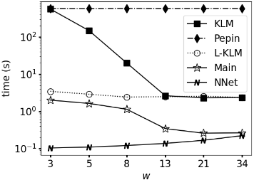
As a baseline, we compared our Main Algorithm directly to reported Neural#DNF running time and previous benchmark regimes in Figure 1. We generated DNFs with n =15,000 (the largest reported by Neural #DNF) and m = 0.75n, with various uniform widths w = 3, 5, 8, 13, 21, 34. Such DNFs are somewhat artificial, with the undesirable property that µ → 1 as n → ∞, but this matches methodology used in the experiments of [Meel et al., 2019] and [Soos et al., 2023] along with the parameter modifications in [Abboud et al., 2020].
Neither Pepin nor L-KLM is significantly affected by the width w, as noted in [Soos et al., 2023]. We speculate that the discrepancy in performance between KLM and Pepin from previous publications is due to the tighter PAC bound requirement. Loose bounds ε = 0.8 and δ = 0.36 were used to benchmark Pepin; the ε, δ scaling observed from Figure 4a as well as the extra log(1/ε) factors in the complexity bounds of Table 2 indicate that Pepin will become much slower for the tighter bounds ε = 0.1, δ = 0.05.
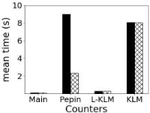
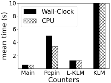
We mention that most previous benchmarks had reported CPU time, but we found that this misrepresents the actual time
(a) Mild PAC bounds. ε = 0.2,
δ = 0.1, n = m = 213 .
(b) Loose PAC bounds. ε = 0.5, δ = 0.25, n = m = 217 .
Figure 2: Mean running times for the two regimes on the six different scenarios of uniform width in {3,5,8,13,21,34}.
required. The following experiments shown in Figure 2 show the mean of both wall-clock and CPU time for each method to solve the six benchmark regimes. Because of this issue, aside from Figure 2 all other timing reported is in wall-clock time as opposed to CPU time.
We see that Pepin spends a large proportion of its time waiting on the kernel and that this percentage increases as ε and δ decrease. We speculate this may be due to the larger memory and randomness requirements inherent in Pepin. This provides good reason for us to record our benchmark in wallclock time.
7.2 ANew Family of Benchmarks
One main disadvantage of prior benchmarks, where the clauses are generated independently, is that for large instances the satisfaction probability µ approaches to one. For such problems, much simpler algorithms based on naive Monte Carlo estimation could be used instead.
To attempt to better capture hard large-scale problem instances, we generate a new family of synthetic formulas inspired by [Meel et al., 2019] and [Abboud et al., 2020]. Each formula is randomly generated with a specified n and m beforehand, and has a small number of "stems", i.e. a selection of randomly chosen variables shared among many clauses. For each distinct clause, the amount of variables added to its stem is randomly chosen. Finally, each variable in the clause is set according to ρ. Details are found in Procedure P2 below.
Procedure P2
Require: Integers n,m, α, γ, λ > 0.
- 1: Initialize Φ← ∅.
- 2: while |Φ| <mdo
- 3: Form a stemCσ by choosing γ variables at random and assigning them according to ρ.
- 4: for t = 1, . . . ,m/α do
- 5: Choose a width w′ uniformly in {1, . . . , λ}.
- 6: C ←Cσ.
- 7: for i = 1 to w′ do
- 8: Randomly assign a randomly selected variable v according to ρ.
9:
Add v or ¬v to C.
- 10: Φ←Φ∪ {C}
- 11: return DNF formula Φ.
Here, parameter α specifies the number of stems, γ specifies the number of variables per stem, and λ controls how many variables to add to a stem.
There are two main advantages with the DNFs generated by this process. First is that non-uniform width more accurately represents problems which show up in practice, and second we want to maintain a significant value for p to ensure a similar computational hardness as that of the small uniform width case.
All experiments were conducted on a compute node consisting of a 4× Intel Xeon Platinum 8260 CPUs with 4 × 24 real cores and 1 TB of RAM. All algorithms used a few GB, nowhere near 1 TB. The KLM and L-KLM algorithms were implemented in C++ and compiled with the O3 flag. The Monte Carlo algorithms, including ours, all share the same support functions wherever applicable and use the improved discrete sampling algorithm with Mersenne Twister randomization. We obtained the code for Pepin from the author's Github (version 1.3).
7.3 Scaling DNF Size
We generated DNFs with Procedure P2 for n = 2x , where x = 10, . . . , 27, and parameters
The results are shown in Figure 3.
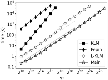
We see that KLM has the worst scaling of all methods, and that Pepin solved the fewest problems before the timeout of 1 day. The experiment demonstrates that our Main Algorithm and L-KLM can solve problem sizes with n > 106 at 95% accuracy. Indeed, our Main Algorithm's work at n = 227 is comparable to KLMs work at n = 217 ; this indicates a longstanding barrier has been broken since Neural#DNF increased feasible sizes to n =15,000 at 90% accuracy. our Main Algorithm also provides more than an order of magnitude speedup compared to L-KLM.
7.4 Scaling the PAC Bounds
For our next experiment, we fixed n = m = 212 , and fixed either ε or δ while the other varied over a wide range. See Figure 4. Note that our Main Algorithm has much better scaling in ε, δ compared to Pepin, and it obtains 99.9% accuracy in comparable time to KLM and Pepin's attainment of 99.0% and 95.0% accuracy respectively.
To test accuracy we generated 32 DNFs with number of variables n ranging from 4 to 32 in increments of 4. For each n, we allowed m to range through { 3 4 , 44 , 54 , 64 } · n. We fixed δ = 0.05 and allowed ε to range in [0.005, 0.1].
Figure 5 shows that all the methods provide the guaranteed accuracy, except for Pepin in smaller problem cases. There seems to be some dependency between the size of the problem and ε for the accuracy guarantee in Pepin. We observe that our Main Algorithm returns a relative accuracy well below the guarantee regardless of problem size.
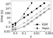
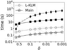
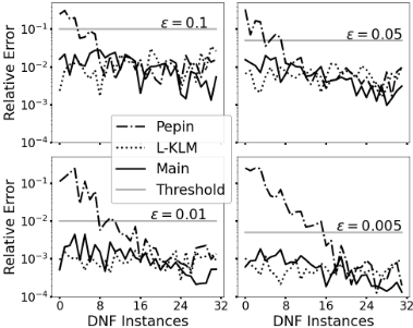
Figure 5: Accuracy Tests. δ = 0.05, ε ∈ [0.005, 0.1]
7.5 Discussion on AlgorithmPerformance
The fact that we outperform all other FPRASs even on uniformwidth DNFs and on small problem sizes, where our permutation heuristic provides little to no benefit, is a testament to the robustness of our approach.
There appear to be a number of distinct reasons for the improved perfomance, with different affects on different types of datasets and different parameter regimes. Here we highlight some factors that we believe explain many of the advantages of our Main Algorithm.
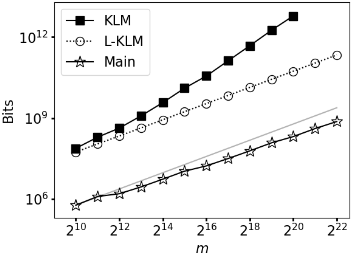
Random sampling. The inner loops of KLM and L-KLM sample Θ(logm) random bits per step, to choose the next clause. By contrast, in our Main Algorithm, the only random samples are needed for the variables. Because we can use short-circuit evaluation of each clause, this only requires O(1) random bits in expectation. Consequently, our Main Algorithm uses much less randomness compared to KLM and L-KLM. While theoretical analysis of algorithms typically assumes access to a random tape in O(1) time, in practice generating (pseudo)-random values can be much more expensive than other arithmetic operations.
In Figure 6, we generated DNFs with procedure P2 and chose α = 8, γ = ⌊ 14 log2 m⌋, and λ = ⌊2 log2 m⌋. We see the significantly reduced and slow growing random number generation in the algorithm.
Memory access pattern. The inner loop of our Main Algorithm is to step through the clauses in a fixed order given by the permutation π. By contrast, in KLM and L-KLM, the clauses must be processed in a uniformly random order. This is one of the worst access patterns for large memory. While the usual asymptotic conventions assume that memory access takes O(1) time, real-world memory times typically vary depending on access locality.
The situation for Pepin is even worse: while KLM, L-KLM and our Main Algorithm handle each trial separately, Pepin must effectively store them all together. As a result, the memory usage scales with problem size as well as ε and δ. For small values of ε, in particular, the working memory may exceed the available low-level memory caches. This can dramatically inflate the running time, and is another reason why our Main Algorithm can be so much faster compared to Pepin.
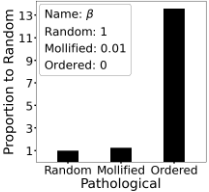
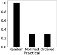
Clause selection heuristic. One key feature of our Main Algorithm is that the permutation π can use heuristics to choose the clause, e.g. by preferentially selecting small clauses. In our asymptotic analysis, we have ignored any potential benefits from the clause-selection heuristic; it is simply taken as a possible surprise bonus in work. As we see in Figure 7, the clause selection with β = 0.01 provides almost all of the theoretical benefits of the random permutation on pathological instances, but also essentially matches the greedy clause-selection heuristic on typical instances.
Variable ordering. A side effect of the consistent clause order is that we can use more compact data structures to represent the variables. This allows further speedups. It also allows us to simplify the code, since we do not need to switch between sparse and dense representations to clear the variables.
Tight PAC Bounds. In both KLM and our Main Algorithm, the average number of trials is Θ( log(1/δ) pε2 ). However, the constant factor for KLM is roughly 4× larger. The main reason for this is that our stopping threshold is defined in terms of Binomial random variables and a Chernoff bound; this is similar to, but slightly tighter than, the generic stopping rule of [Dagum et al., 2000]. By contrast, the threshold for KLM requires more generic bounds in terms of optional stopping for martingales; note that the stopping rule of [Dagum et al., 2000] would not be valid for the KLM algorithm, since the relevant statistic for the KLM algorithm (the waiting time to observe a true clause) is not bounded.
We also mention that the concentration bounds given for Pepin may be erroneous, as shown in Figure 3.
@inproceedings{ijcai2026p244,
  title     = {Scalable Algorithms for Approximate DNF Model Counting},
  author    = {Burkhardt, Paul and Harris, David G. and Schmitt, Kevin T.},
  booktitle = {Proceedings of the Thirty-Fifth International Joint Conference on
               Artificial Intelligence, {IJCAI-26}},
  publisher = {International Joint Conferences on Artificial Intelligence Organization},
  editor    = {Diego Calvanese},
  pages     = {2191--2198},
  year      = {2026},
  month     = {8},
  note      = {Main Track},
  doi       = {10.24963/ijcai.2026/244},
  url       = {https://doi.org/10.24963/ijcai.2026/244},
}
TY - CPAPER TI - Scalable Algorithms for Approximate DNF Model Counting AU - Burkhardt, Paul AU - Harris, David G. AU - Schmitt, Kevin T. T2 - Proceedings of the Thirty-Fifth International Joint Conference on Artificial Intelligence, IJCAI-26 PB - International Joint Conferences on Artificial Intelligence Organization PY - 2026 SP - 2191 EP - 2198 DO - 10.24963/ijcai.2026/244 UR - https://doi.org/10.24963/ijcai.2026/244 ER -Copied
Machine-readable versions of this paper, for tools and AI agents:





