
Student-t Variational Autoencoder for Robust Density Estimation
Proceedings of the Twenty-Seventh International Joint Conference on Artificial Intelligence. Main track. Pages 2696-2702.
https://doi.org/10.24963/ijcai.2018/374
Keywords
- Machine Learning: Neural Networks
- Machine Learning: Machine Learning
- Machine Learning: Deep Learning
- Machine Learning: Probabilistic Machine Learning
- Machine Learning: Unsupervised Learning
Abstract
We propose a robust multivariate density estimator based on the variational autoencoder (VAE). The VAE is a powerful deep generative model, and used for multivariate density estimation. With the original VAE, the distribution of observed continuous variables is assumed to be a Gaussian, where its mean and variance are modeled by deep neural networks taking latent variables as their inputs. This distribution is called the decoder. However, the training of VAE often becomes unstable. One reason is that the decoder of VAE is sensitive to the error between the data point and its estimated mean when its estimated variance is almost zero. We solve this instability problem by making the decoder robust to the error using a Bayesian approach to the variance estimation: we set a prior for the variance of the Gaussian decoder, and marginalize it out analytically, which leads to proposing the Student-t VAE. Numerical experiments with various datasets show that training of the Student-t VAE is robust, and the Student-t VAE achieves high density estimation performance.
- [Burda et al., 2015] Yuri Burda, Roger Grosse, and Ruslan Salakhutdinov. Importance weighted autoencoders. arXiv preprint arXiv:1509.00519, 2015.
- [Duchi et al., 2011] John Duchi, Elad Hazan, and Yoram Singer. Adaptive subgradient methods for online learning and stochastic optimization. Journal of Machine Learning Research, 12(Jul):2121-2159, 2011.
- [Geusebroek et al., 2005] Jan-Mark Geusebroek, Gertjan J Burghouts, and Arnold WM Smeulders. The amsterdam library of object images. International Journal of Com- puter Vision, 61(1):103-112, 2005.
- [Goldstein and Uchida, 2016] Markus Goldstein and Seiichi Uchida. A comparative evaluation of unsupervised anomaly detection algorithms for multivariate data. PloS one, 11(4):e0152173, 2016.
- [Goodfellow et al., 2016] Ian Goodfellow, Yoshua Bengio, and Aaron Courville. Deep Learning. MIT Press, 2016. http://www.deeplearningbook.org. Link
- [Johnson and Zhang, 2013] Rie Johnson and Tong Zhang. Accelerating stochastic gradient descent using predictive variance reduction. In Advances in neural information pro- cessing systems, pages 315-323, 2013.
- [Jylänki et al., 2011] Pasi Jylänki, Jarno Vanhatalo, and Aki Vehtari. Robust Gaussian process regression with a Student-t likelihood. Journal of Machine Learning Re- search, 12(Nov):3227-3257, 2011.
- [Kingma and Ba, 2014] Diederik Kingma and Jimmy Ba. Adam: A method for stochastic optimization. arXiv preprint arXiv:1412.6980, 2014.
- [Kingma and Welling, 2013] Diederik P Kingma and Max Welling. Auto-encoding variational Bayes. arXiv preprint arXiv:1312.6114, 2013.
- [Kingma et al., 2015] Diederik P Kingma, Tim Salimans, and Max Welling. Variational dropout and the local repa- rameterization trick. In Advances in Neural Information Processing Systems, pages 2575-2583, 2015.
- [Lange et al., 1989] Kenneth L Lange, Roderick JA Little, and Jeremy MG Taylor. Robust statistical modeling us- ing the t distribution. Journal of the American Statistical Association, 84(408):881-896, 1989.
- [Lichman, 2013] M. Lichman. UCI machine learning repos- itory, 2013.
- [Maaten and Hinton, 2008] Laurens van der Maaten and Ge- offrey Hinton. Visualizing data using t-SNE. Journal of Machine Learning Research, 9(Nov):2579-2605, 2008.
- [Martinez-Cantin et al., 2017] Ruben Martinez-Cantin, Michael McCourt, and Kevin Tee. Robust Bayesian optimization with Student-t likelihood. arXiv preprint arXiv:1707.05729, 2017.
- [McLachlan and Peel, 2004] Geoffrey McLachlan and David Peel. Finite mixture models. John Wiley & Sons, 2004.
- [Miller et al., 2017] Andrew Miller, Nick Foti, Alexander D'Amour, and Ryan P Adams. Reducing reparameteriza- tion gradient variance. In Advances in Neural Information Processing Systems 30, pages 3711-3721, 2017.
- [Pedregosa et al., 2011] Fabian Pedregosa, Gaël Varoquaux, Alexandre Gramfort, Vincent Michel, Bertrand Thirion, Olivier Grisel, Mathieu Blondel, Peter Prettenhofer, Ron Weiss, Vincent Dubourg, et al. Scikit-learn: Machine learning in Python. Journal of Machine Learning Re- search, 12(Oct):2825-2830, 2011.
- [Rezende et al., 2014] Danilo J Rezende, Shakir Mohamed, and Daan Wierstra. Stochastic backpropagation and ap- proximate inference in deep generative models. In Pro- ceedings of the 31st International Conference on Machine Learning, pages 1278-1286, 2014.
- [Roeder et al., 2017] Geoffrey Roeder, Yuhuai Wu, and David K Duvenaud. Sticking the landing: Simple, lower-variance gradient estimators for variational infer- ence. In Advances in Neural Information Processing Sys- tems, pages 6928-6937, 2017.
- [Scott, 2015] David W Scott. Multivariate density estima- tion: theory, practice, and visualization. John Wiley & Sons, 2015.
- [Silverman, 1986] Bernard W Silverman. Density estimation for statistics and data analysis, volume 26. CRC press, 1986.
- [Suh et al., 2016] Suwon Suh, Daniel H Chae, Hyon-Goo Kang, and Seungjin Choi. Echo-state conditional varia- tional autoencoder for anomaly detection. In Neural Net- works (IJCNN), 2016 International Joint Conference on, pages 1015-1022. IEEE, 2016.
- [Tieleman and Hinton, 2012] Tijmen Tieleman and Geoffrey Hinton. Lecture 6.5-rmsprop: Divide the gradient by a running average of its recent magnitude. COURSERA: Neural networks for machine learning, 4(2):26-31, 2012.
- [van den Oord et al., 2016] Aaron van den Oord, Nal Kalch- brenner, Lasse Espeholt, Oriol Vinyals, Alex Graves, et al. Conditional image generation with PixelCNN decoders. In Advances in Neural Information Processing Systems, pages 4790-4798, 2016.
- [Wang et al., 2013] Chong Wang, Xi Chen, Alexander J Smola, and Eric P Xing. Variance reduction for stochastic gradient optimization. In Advances in Neural Information Processing Systems, pages 181-189, 2013.
- [Zeiler, 2012] Matthew D Zeiler. ADADELTA: an adaptive learning rate method. arXiv preprint arXiv:1212.5701, 2012.
References were extracted automatically from the PDF and may contain errors.
Full text extracted automatically from the PDF; figures, tables and equations may differ. The PDF is the version of record.
1 Introduction
Multivariate density estimation [Scott, 2015], which estimates the distribution of continuous data, is an important task for artificial intelligence. This fundamental task is widely performed from basic analysis such as clustering and data visualization to applications such as image processing, speech recognition, natural language processing, and anomaly detection. For these tasks, conventional density estimation methods such as the kernel density estimation [Silverman, 1986] and the Gaussian mixture model [McLachlan and Peel, 2004] are often used. However, recent developments of networks and sensors have made data more high-dimensional, complicated, and noisy, and hence multivariate density estimation has become very difficult.
Meanwhile, the variational autoencoder (VAE) [Kingma and Welling, 2013; Rezende et al., 2014] was presented as a powerful generative model for learning high-dimensional complicated data by using neural networks, and the VAE is used for multivariate density estimation. The VAE is composed of two conditional distributions: the encoder and the decoder, where neural networks are used to model the parameters of these conditional distributions. The encoder infers the posterior distribution of continuous latent variables given an observation. The decoder infers the posterior distribution of observation given a latent variable. The encoder and decoder neural networks are optimized by minimizing the training objective function. In the density estimation task, since the observed variables are continuous, a Gaussian distribution is used for the decoder. We call this type of VAE the Gaussian VAE.
However, the training of the Gaussian VAE often becomes unstable. The reason is as follows: the training objective function of Gaussian VAE is sensitive to the error between the data point and its decoded mean when its decoded variance is almost zero, and hence, the objective function can give an extremely large value even with a small error. We call this problem zero-variance problem. This zero-variance problem often occurs with biased data, i.e. in which some clusters of data points have small variance. Real-world datasets such as network, sensor and media datasets often have this bias, therefore, this problem is serious considering the application of the VAE for real-world datasets.
Our purpose is to solve this instability by making the decoder robust to the error. In this paper, we introduce a Bayesian approach to the inference of the Gaussian decoder: we set a Gamma prior for the inverse of the variance of the decoder and marginalize it out analytically, which leads to introducing a Student-t distribution as the decoder distribution. We call this proposed method the Student-t VAE. Since the Student-t distribution is a heavy-tailed distribution [Lange et al., 1989], the Student-t decoder is robust to the error between the data point and its decoded mean, which makes the training of the Student-t VAE stable.
2 Variational Autoencoder
First, we review the variational autoencoder (VAE) [Kingma and Welling, 2013; Rezende et al., 2014]. The VAE is a probabilistic latent variable model that relates an observed variable vector x to a continuous latent variable vector z by a conditional distribution. Since our task is density estimation, we assume that the observed variables x are continuous. With the VAE, the probability of a data point x is given by
where p (z) is a prior of the latent variable vector, which is usually modeled by a standard Gaussian distribution N (z|0, I), and pθ (x|z) = N (x | µθ (z) , σ2 θ (z)) is a Gaussian distribution with mean µθ (z) and variance σ2 θ (z), which are modeled by neural networks with parameter θ and input z. These neural networks are called the decoder. We call this type of VAE the Gaussian VAE.
Given a dataset X = {x(1) , . . . , x(N)}, the sum of the marginal log-likelihoods is given by
where N is the number of data points. The marginal loglikelihood is bounded below by the variational lower bound, which is derived from Jensen's inequality, as follows:
where E[·] represents the expectation, qφ (z | x) = N (z | µφ (x) , σ2φ (x)) is the posterior of z given x, and its mean µφ (x) and variance σ2φ (x) are modeled by neural networks with parameter φ. These neural networks are called the encoder.
The variational lower bound (3) can be also written as:
where DKL (P‖Q) is the Kullback Leibler (KL) divergence between P and Q. The parameters of the encoder and decoder neural networks are optimized by maximizing the variational lower bound using stochastic gradient descent (SGD) [Duchi et al., 2011; Zeiler, 2012; Tieleman and Hinton, 2012; Kingma and Ba, 2014]. The expectation term in (4) is approximated by the reparameterization trick [Kingma and Welling, 2013]:
where z(i,ℓ) = µφ (x(i) ) + ε(i,ℓ)σ2φ (x(i) ), ε(i,ℓ) is a sample drawn fromN (0, I), and L is the sample size of the reparameterization trick. L = 1 is usually used [Kingma and Welling,
2013]. Then, the resulting objective function is
The KL divergence between Gaussian distributions DKL (qφ (z | x(i) ) ‖p (z)) and its gradient can be calculated analytically [Kingma and Welling, 2013]. In this paper, we minimize the negative of (6) instead of maximizing it.
3 Instability of Training Gaussian VAE
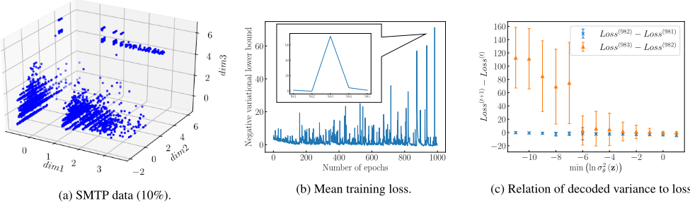
To investigate the Gaussian VAE, we applied it to SMTP data 1 , which is a subset of the KDD Cup 1999 data and provided by the scikit-learn community [Pedregosa et al., 2011]. The KDD Cup 1999 data were generated using a closed network and hand-injected attacks for evaluating the performance of supervised network intrusion detection, and they have often been used also for unsupervised anomaly detection. The SMTP data consists of three-dimensional continuous data, and contains 95,156 data points. Figure 1a shows a visualization of this dataset. This dataset has some bias: the variance of some clusters of data points is small along the dimension directions.
We trained the Gaussian VAE using this dataset by Adam [Kingma and Ba, 2014] with mini-batch size of 100. We used a two-dimensional latent variable vector z, two-layer neural networks (500 hidden units per layer) as the encoder and the decoder, and a hyperbolic tangent as the activation function. The data were standardized with zero mean and unit variance. We used 10% of this dataset for training.
Figure 1b shows the mean training loss, which equals - ∑Ni=1 ˆ L (θ, φ; x(i) ) /N. The training loss was very unstable. One reason for this is that the variance σ2 θ (z(i,ℓ) ) in the decoder N (x(i) |µθ (z(i,ℓ) ) , σ2 θ (z(i,ℓ) )) becomes almost zero, where z(i,ℓ) is sampled from the encoder N (z(i,ℓ) |µφ (x(i) ) , σ2φ (x(i) )). For example, at the 983rd epoch, the training loss jumped up sharply. Figure 1c shows the relationship between the difference in the training losses and the variance σ2 θ (z(i,ℓ) ) at this epoch. The training loss of the data points with small variance σ2 θ (z(i,ℓ) ) increased drastically.
When the decoded variance σ2 θ (z(i,ℓ) ) is almost zero, the Gaussian decoder is sensitive to the error between the data point and its decoded mean: even if x(i) differs only slightly from its decoded mean µθ (z(i,ℓ) ), the value of the first term of the training objective function (6):
1 This dataset is available at http://scikit-learn.org/stable/ modules/generated/sklearn.datasets.fetch kddcup99.html
changes drastically, where d is the dimension index of x(i) , µθ (z(i,ℓ) ), and σ2 θ (z(i,ℓ) ). This sensitivity makes the training of the Gaussian VAE unstable. We call this problem the zero-variance problem. This zero-variance problem often occurs with biased data, since some data points are from a cluster with very small variance, and their decoded variance becomes much smaller as the training proceeds. Since the cause of this problem is the sensitivity of the objective function, changing the optimizer and tuning the hyperparameters of optimizer do not matter.
4 Student-t VAE
We would like to solve this zero-variance problem by making the decoder robust to the error between the data point and its decoded mean. We propose a Bayesian approach to the inference of the Gaussian decoder, which leads to using a Student-t distribution as the decoder.
We introduce a prior distribution for the variance of the Gaussian decoder. Let the precision parameter τθ(z) be the inverse of the variance, τθ(z) = 1/σ2 θ (z). We use the conjugate prior for the precision parameter, which is the following Gamma distribution:
where a is a shape parameter and b is a rate parameter. The domains of a and b are positive.
4.1 MAP Estimation
First, we present the maximum a posteriori (MAP) estimation as a way to solve the zero-variance problem. To simplify the calculation, we use Gam(τ | 1, b) as the prior for 1/σ2 θ (z). Its log probability is given by
Accordingly, the objective function of MAP estimation for the VAE is:
We call this type of VAE the MAP VAE. This objective function can be viewed as a regularized version of the original Gaussian VAE objective function (6), where the small variance σ2 θ (z(i,ℓ) ) is penalized by -b/σ2 θ (z(i,ℓ) ) with the regularization parameter b. This regularization parameter b can be tuned by cross-validation, which requires a heavy computational cost. In addition, the MAP VAE has a problem in that the prior distribution is assumed to be independent of latent variables z, which leads to a lack of flexibility in density estimation.
4.2 Marginalization of the Variance Parameter
We propose a more flexible and computationally efficient approach by introducing a Gamma prior distribution that depends on latent variables, Gam(τ | a (z) , b (z)), where a (z) and b (z) are the shape and rate parameters, respectively, which take the latent variable z as their inputs. By analytically integrating out the precision τ, the conditional distribution of the observation x given the latent variable z becomes
𝜇𝜃 𝐳
𝐱
𝜎𝜃2 𝐳
𝐳
(a) Gaussian decoder.
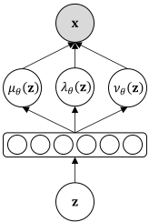
Figure 2: The diagram of decoders. The decoder neural network takes the latent variable z as input, and estimates the parameters of assumed distribution. (a) Gaussian decoder network estimates the mean µθ (z) and variance σ2 θ (z). (b) Student-t decoder network estimates the mean µθ (z), precision λθ (z), and degree of freedom νθ (z).
a Student-t distribution as follows:
where λθ (z) = a(z)/b (z) is a precision 2 of a Student-t distribution, and νθ (z) = 2a (z) is a degree of freedom. We use neural networks to model the parameters of the Student-t distribution, λθ (z) and νθ (z) as well as µθ (z), and use them as the decoder. We call this type of VAE the Student-t VAE. The diagram of Student-t decoder is illustrated in Figure 2.
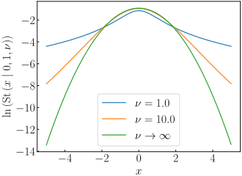
Figure 3 shows a plot of the Student-t distribution. The Student-t distribution is obtained by mixing an infinite number of Gaussians that have the same mean but different variances, and it has an important property: the tail heaviness. It is well-known that a heavy-tailed distribution is robust because the probability in the tail region is higher than that of a light-tailed distribution such as a Gaussian distribution [Lange et al., 1989]. Therefore, the Student-t decoder is robust to the error between the data point and its decoded mean, which makes the training of the Student-t VAE stable. Since the degree of tail heaviness can be adjusted by tuning ν, the Student-t VAE can set an appropriate robustness for each data point by estimating νθ (z), which leads to obtaining better flexibility than the MAP VAE. Since there is no need to use the cross-validation for tuning the parameters such as the MAP VAE, the Student-t VAE requires only a lightweight computational cost.
2 This parameter is not always equal to the inverse of the variance.
| SMTP | Aloi | Thyroid | Cancer | Satellite | |
|---|---|---|---|---|---|
| Data size | 95,156 | 50,000 | 6,916 | 367 | 5,100 |
| Dimension | 3 | 27 | 21 | 30 | 36 |
5 Experiments
In this section, we evaluate the robustness of the training and the density estimation performance of the Student-t VAE.
5.1 Data
We used the following five datasets: SMTP, Aloi, Thyroid, Cancer and Satellite. The SMTP data is the same as the data used in Section 3, where we used 10% of this dataset for training. We also used 10% of this dataset for validation and the remaining 80% for test. The Aloi data is the Amsterdam library of object images [Geusebroek et al., 2005], and the Thyroid, Cancer and Satellite datasets were obtained from the UCI Machine Learning Repository [Lichman, 2013]. We used the transformations of these datasets by [Goldstein and Uchida, 2016] 3 . We used 50% of the dataset for training, 10% for validation, and the remaining 40% for test. The total number of data points and the dimensions of the observation of the five datasets are listed in Table 1.
5.2 Setup
We used two-layer neural networks (500 hidden units per layer) as the encoder and the decoder, and a hyperbolic tangent as the activation function. We trained the VAE by using Adam [Kingma and Ba, 2014] with mini-batch size of 100. We set the sample size of the reparameterization trick to L = 1. The maximum number of epochs was 500, and we used early-stopping [Goodfellow et al., 2016] based on the validation data. We used a two-dimensional latent variable vector z with the SMTP data, and a 20-dimensional latent
3 These datasets are available at https://dataverse.harvard.edu/ dataset.xhtml?persistentId=doi:10.7910/DVN/OPQMVF
| Method | SMTP | Aloi | Thyroid | Cancer | Satellite |
|---|---|---|---|---|---|
| Gaussian | -1.248 ± 0.404 | 45.418 ± 5.457 | 15.519 ± 4.422 | -18.668 ± 3.448 | -1.852 ± 0.370 |
| MAP(b = 1) | -4.864 ± 0.020 | -38.210 ± 0.156 | -31.266 ± 0.159 | -45.895 ± 0.843 | -50.895 ± 0.238 |
| MAP(b = 0.001) | -1.932 ± 0.404 | 30.406 ± 0.383 | 18.037 ± 1.318 | -19.017 ± 3.273 | -1.899 ± 0.372 |
| Student-t | 0.827 0.105 | 77.022 0.539 | 69.543 0.634 | -18.253 2.629 | -1.811 0.289 |
0.827 ± 0.105 77.022 ± 0.539 69.543 ± 0.634 -18.253 ± 2.629 -1.811 ± 0.289
Table 2: Comparison of test log-likelihoods. We highlighted the best result in bold, and we also highlighted the results in bold which are not statistically different from the best result according to a pair-wise t-test. We use 5% as p-value.
variable vector for the other datasets. For the evaluation, we calculated the marginal log-likelihood of the test data by using the importance sampling [Burda et al., 2015]. We set the sample size of the importance sampling to 100. We ran all experiments ten times each. The data was standardized with zero mean and unit variance. We used the following setup: CPU was Intel Xeon E5-2640 v4 2.40GHz, the memory size was 1 TB, and GPU was NVIDIA Tesla M40.
5.3 Results
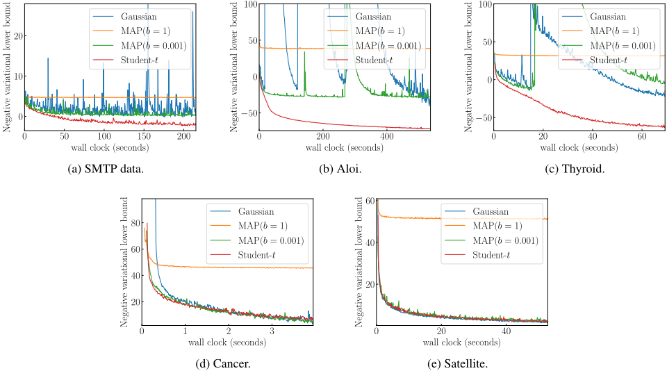
Figures 4a-4e show the relationship between the mean training loss and wall clock (seconds), and Table 2 compares the test log-likelihoods of the Gaussian VAE, MAP VAE, and Student-t VAE.
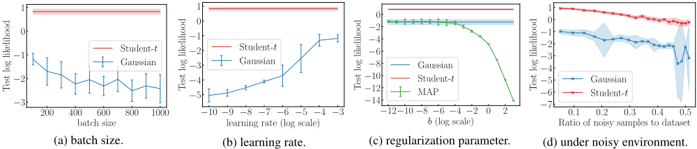
First, we focused on the Gaussian VAE. With the SMTP, Aloi and Thyroid data, training of the Gaussian VAE was unstable, and the test log-likelihoods of the Gaussian VAE were worse than those of the Student-t VAE. On the other hand, with the Cancer and Satellite data, the training of the Gaussian VAE was stable, and the Gaussian VAE and the Student-t VAE achieved the comparable test log-likelihoods. Figures 5a and 5b show the test log-likelihoods by the Gaussian VAE for different mini-batch sizes, and different learning rates for the SMTP data, respectively. Even though the mini-batch size and learning rate changed, the test log-likelihood with the Gaussian VAE was worse than that with the Student-t VAE. These results indicate that improving the robustness of the objective function is better than tuning the hyper parameters of the optimizer.
Second, we focused on the MAP VAE. When the regularization parameter was large, b = 1, the negative variational lower bound was stable but it did not decrease well. When the regularization parameter was small, b = 0.001 with the SMTP, Aloi and Thyroid data, the negative variational lower bound became unstable, and it behaved similarly to that of the Gaussian VAE. The test log-likelihoods of the MAP VAE were equal to or worse than the Gaussian VAE, because the constant parameter of the Gamma prior b was not flexible. Figure 5c shows the test log-likelihoods with different regularization parameter values b for the SMTP data. When b ≤ 0.001, the test log-likelihood of the MAP VAE was not statistically different from the Gaussian VAE, and when b ≥ 0.01, the larger b was, the worse the test log-likelihood of the MAP VAE became. These results indicate that setting an appropriate robustness for each data point is effective to avoid zero-variance problem without lacking the flexibility of density estimation.
Third, we focused on the Student-t VAE. With all of the datasets, the Student-t VAE reduced the training loss stably, and obtained the equal to or better density estimation performance than that of the Gaussian VAE and the MAP VAE. Since the Student-t VAE can set the appropriate robustness for each data point by estimating νθ (z), it avoids zero-variance problem while improving the flexibility of the decoder, which makes the training stable and leads to obtaining good density estimation performance.
In addition, we evaluated the stability of training under the noisy environment. We added noisy samples which follows uniform distribution to SMTP data, and evaluated the test loglikelihoods. Figure 5d shows the relationship between the test log-likelihoods and the ratio of noisy samples to dataset. Whereas the training of Gaussian VAE becomes unstable as the ratio of noisy samples increases, the training of Studentt VAE continues to be stable. This result indicates that the Student-t VAE is useful under the noisy environments such as real-world applications.
These results indicate that the Student-t VAE is a good alternative to the Gaussian VAE: the training of the Studentt VAE is stable, which requires only a lightweight computational cost, and the density estimation performance of the Student-t VAE is equal to or better than that of the Gaussian VAE.
6 RelatedWork
Regarding related work on improving the stability of training the VAE, a number of methods have been proposed that reduce the variance of stochastic gradients [Johnson and Zhang, 2013; Wang et al., 2013; Kingma et al., 2015;
Roeder et al., 2017; Miller et al., 2017]. These methods focused on the stability of optimization methods, such as the reparameterization trick and the stochasticity due to data subsampling. The Student-t VAE focuses on the different part from these methods: the robustness of the training objective function. This requires only a lightweight computational cost, and can be used together with these existing methods.
It is well-known that the Student-t distribution has robustness [Lange et al., 1989], and this robustness has been applied to a number of machine learning algorithms, such as stochastic neighbor embedding [Maaten and Hinton, 2008], Gaussian process [Jyl¨anki et al., 2011], and Bayesian optimization [Martinez-Cantin et al., 2017]. These algorithms used a Student-t distribution to reduce the influence of noise included in the observed data. The Student-t VAE uses a Student-t distribution for reducing the influence of the error between the data point and its decoded mean, which makes the training objective function of Student-t VAE robust.
7 Conclusion
We proposed the Student-t variational autoencoder: a robust multivariate density estimator based on the variational autoencoder (VAE). The training of the Gaussian VAE often becomes unstable. We investigated the cause of this instability, and revealed that the Gaussian decoder is sensitive to the error between the data point and its decoded mean when the decoded variance is almost zero.
In order to improve the robustness of the VAE, we introduced a Bayesian approach to the Gaussian decoder: we set a Gamma prior for the inverse of the decoded variance and marginalized it out analytically, which led to using the Student-t distribution as the decoder. Since the Student-t distribution is a heavy-tailed distribution, the Student-t decoder is robust to the error, which makes the training stable. We demonstrated that the robustness of the training and the high density estimation performance of the Student-t VAE in experiments using five datasets.
In the future, we will try to apply the Student-t VAE to real-world applications such as anomaly detection [Suh et al., 2016] and image generation [van den Oord et al., 2016].
@inproceedings{ijcai2018p374,
  title     = {Student-t Variational Autoencoder for Robust Density Estimation},
  author    = {Takahashi, Hiroshi and Iwata, Tomoharu and Yamanaka, Yuki and Yamada, Masanori and Yagi, Satoshi},
  booktitle = {Proceedings of the Twenty-Seventh International Joint Conference on
               Artificial Intelligence, {IJCAI-18}},
  publisher = {International Joint Conferences on Artificial Intelligence Organization},
  editor    = {Jérôme Lang},
  pages     = {2696--2702},
  year      = {2018},
  month     = {7},
  note      = {Main track},
  doi       = {10.24963/ijcai.2018/374},
  url       = {https://doi.org/10.24963/ijcai.2018/374},
}
TY - CPAPER TI - Student-t Variational Autoencoder for Robust Density Estimation AU - Takahashi, Hiroshi AU - Iwata, Tomoharu AU - Yamanaka, Yuki AU - Yamada, Masanori AU - Yagi, Satoshi T2 - Proceedings of the Twenty-Seventh International Joint Conference on Artificial Intelligence, IJCAI-18 PB - International Joint Conferences on Artificial Intelligence Organization PY - 2018 SP - 2696 EP - 2702 DO - 10.24963/ijcai.2018/374 UR - https://doi.org/10.24963/ijcai.2018/374 ER -Copied
Machine-readable versions of this paper, for tools and AI agents:





