
Latent Semantics Encoding for Label Distribution Learning
Proceedings of the Twenty-Eighth International Joint Conference on Artificial Intelligence. Main track. Pages 3982-3988.
https://doi.org/10.24963/ijcai.2019/553
Keywords
- Machine Learning: Data Mining
- Machine Learning: Feature Selection ; Learning Sparse Models
- Machine Learning: Multi-instance;Multi-label;Multi-view learning
- Machine Learning: Classification
Abstract
Label distribution learning (LDL) is a newly arisen learning paradigm to deal with label ambiguity problems, which can explore the relative importance of different labels in the description of a particular instance. Although some existing LDL algorithms have achieved better effectiveness in real applications, most of them typically emphasize on improving the learning ability by manipulating the label space, while ignoring the fact that irrelevant and redundant features exist in most practical classification learning tasks, which increase not only storage requirements but also computational overheads. Furthermore, noises in data acquisition will bring negative effects on the generalization performance of LDL algorithms. In this paper, we propose a novel algorithm, i.e., Latent Semantics Encoding for Label Distribution Learning (LSE-LDL), which learns the label distribution and implements feature selection simultaneously under the guidance of latent semantics. Specifically, to alleviate noise disturbances, we seek and encode discriminative original physical/chemical features into advanced latent semantic features, and then construct a mapping from the encoded semantic space to the label space via empirical risk minimization. Empirical studies on 15 real-world data sets validate the effectiveness of the proposed algorithm.
- [Berger et al., 1996] Adam L. Berger, Vincent J. Della Pietra, and Stephen A. Della Pietra. A maximum entropy approach to natural language processing. Computational Linguistics, 22(1):39-71, 1996.
- [Boutell et al., 2004] Matthew R. Boutell, Jiebo Luo, X- ipeng Shen, and Christopher M. Brown. Learning multi-label scene classification. Pattern Recognition, 37(9):1757-1771, 2004.
- [Cha, 2007] Sung-Hyuk Cha. Comprehensive survey on distance/similarity measures between probability density functions. International Journal of Mathematical Models and Methods in Applied Sciences, 1(4):300-307, 2007.
- [Della Pietra et al., 1997] Stephen A. Della Pietra, Vincent J. Della Pietra, and John D. Lafferty. Inducing features of random fields. IEEE Transactions on Pattern Analysis and Machine Intelligence, 19(4):380-393, 1997.
- [Demšar, 2006] Janez Demšar. Statistical comparisons of classifiers over multiple data sets. Journal of Machine Learning Research, 7:1-30, 2006.
- [Friedman, 1940] Milton Friedman. A comparison of alter- native tests of significance for the problem of m rankings. The Annals of Mathematical Statistics, 11(1):86-92, 1940.
- [Geng and Hou, 2015] Xin Geng and Peng Hou. Pre-release prediction of crowd opinion on movies by label distribu- tion learning. In Proceedings of the 24th Internation- al Joint Conference on Artificial Intelligence (IJCAI'15), pages 3511-3517, Buenos Aires, Argentina, July 2015.
- [Geng and Ji, 2013] Xin Geng and Rongzi Ji. Label distri- bution learning. In Proceedings of the 13th IEEE Interna- tional Conference on Data Mining Workshops (ICDM'13), pages 377-383, Dallas, Texas, USA, December 2013.
- [Geng et al., 2010] Xin Geng, Kate Smith-Miles, and Zhi- Hua Zhou. Facial age estimation by learning from label distributions. In Proceedings of the 24nd AAAI Confer- ence on Artificial Intelligence (AAAI'10), pages 451-456, Atlanta, Georgia, USA, July 2010.
- [Geng et al., 2013] Xin Geng, Chao Yin, and Zhi-Hua Zhou. Facial age estimation by learning from label distribution- s. IEEE Transactions on Pattern Analysis and Machine Intelligence, 35(10):2401-2412, 2013.
- [Geng, 2016] Xin Geng. Label distribution learning. IEEE Transactions on Knowledge and Data Engineering, 28(7):1734-1748, 2016.
- [Gibaja Galindo and Ventura, 2014] Eva L. Gibaja Galindo and Sebastián Ventura. Multi-label learning: a review of the state of the art and ongoing research. Wiley Interdisci- plinary Reviews: Data Mining and Knowledge Discovery, 4(6):411-444, 2014.
- [Guo et al., 2019] Yumeng Guo, Fulai Chung, Guozheng Li, Jiancong Wang, and James C. Gee. Leveraging label- specific discriminant mapping features for multi-label learning. ACM Transactions on Knowledge Discovery from Data, 13(2):24:1-24:23, 2019.
- [Huang and Zhou, 2012] Sheng-Jun Huang and Zhi-Hua Zhou. Multi-label learning by exploiting label correlations Locally. In Proceedings of the 26th AAAI Conference on Artificial Intelligence (AAAI'12), pages 949-955, Toronto, Ontario, Canada, July 2012.
- [Jia et al., 2018] Xiuyi Jia, Weiwei Li, Junyu Liu, and Yu Zhang. Label distribution learning by exploiting la- bel correlations. In Proceedings of the 32nd AAAI Con- ference on Artificial Intelligence (AAAI'18), pages 3310- 3317, New Orleans, Louisiana, USA, February 2018.
- [Jian et al., 2016] Ling Jian, Jundong Li, Kai Shu, and Huan Liu. Multi-label informed feature selection. In Proceed- ings of the 25th International Joint Conference on Artifi- cial Intelligence (IJCAI'16), pages 1627-1633, New York, NY, USA, July 2016.
- [Liu and Motoda, 1998] Huan Liu and Hiroshi Motoda. Fea- ture Selection for Knowledge Discovery and Data Mining. Kluwer Academic Publishers, Norwell, MA, USA, 1998.
- [Nie et al., 2010] Feiping Nie, Heng Huang, Xiao Cai, and Chris H. Ding. Efficient and robust feature selection vi- a joint ℓ 2,1 -norms minimization. In Proceedings of the 23rd International Conference on Neural Information Pro- cessing Systems (NIPS'10), pages 1813-1821, Vancouver, British Columbia, Canada, December 2010.
- [Nocedal and Wright, 2006] Jorge Nocedal and Stephen J. Wright. Numerical Optimization, 2nd edition. Springer, New York, NY, USA, 2006.
- [Xu et al., 2016] Suping Xu, Xibei Yang, Hualong Yu, Dong-Jun Yu, Jingyu Yang, and Eric C. C. Tsang. Multi-label learning with label-specific feature reduction. Knowledge-Based Systems, 104:52-61, 2016.
- [Yu and Liu, 2004] Lei Yu and Huan Liu. Efficient feature s- election via analysis of relevance and redundancy. Journal of Machine Learning Research, 5:1205-1224, 2004.
- [Zhang and Zhou, 2014] Min-Ling Zhang and Zhi-Hua Zhou. A review on multi-label learning algorithms. IEEE Transactions on Knowledge and Data Engineering, 26(8):1819-1837, 2014.
- [Zhang et al., 2018] Min-Ling Zhang, Yu-Kun Li, Xu-Ying Liu, and Xin Geng. Binary relevance for multi-label learning: an overview. Frontiers of Computer Science, 12(2):191-202, 2018.
- [Zhao and Zhou, 2018] Peng Zhao and Zhi-Hua Zhou. La- bel distribution learning by optimal transport. In Proceed- ings of the 32nd AAAI Conference on Artificial Intelligence (AAAI'18), pages 4506-4513, New Orleans, Louisiana, USA, February 2018.
- [Zhou et al., 2015] Ying Zhou, Hui Xue, and Xin Geng. E- motion distribution recognition from facial expressions. In Proceedings of the 23rd ACM international conference on Multimedia (MM'15), pages 1247-1250, Brisbane, Aus- tralia, October 2015.
References were extracted automatically from the PDF and may contain errors.
Full text extracted automatically from the PDF; figures, tables and equations may differ. The PDF is the version of record.
1 Introduction
Learning with label ambiguity has increasingly attracted attention in recent machine learning and data mining areas. At present, single-label learning (SLL) and multi-label learning (MLL) [Gibaja Galindo and Ventura, 2014; Zhang and Zhou, 2014; Zhang et al., 2018] are two widely-used paradigms to deal with the label ambiguity problems, where each instance only belongs to a single label in SLL, whereas each instance may be associated to multiple labels simultaneously in MLL. Although SLL and MLL have achieved a lot of success [Boutell et al., 2004; Huang and Zhou, 2012] in classification learning tasks, both of them focus on a relatively broad label ambiguity problem, i.e., "which labels can describe a particular instance?", thus the output of an SLL/MLL algorithm often is a set of labels with the implicit assumption that these labels are considered to be equally important. However, sometimes ones need to deal with the further label ambiguity problem of "to what extent will different labels describe a particular instance?", in other words, the relative importance of different labels involved in the description of an instance, i.e., a distribution over the set of labels, is expected to be obtained. For example, a facial expression usually is constituted by a variety of different emotional components, such as dejection, pleasure, enthusiasm and so on. Different emotional components make different contributions to building a particular facial expression, and they form an emotion distribution [Zhou et al., 2015] for facial expression. To solve such learning problems with label ambiguity, [Geng and Ji, 2013] first proposed the concept of label distribution learning (LDL), which can be viewed as a more generalized learning paradigm when compared with the traditional SLL and MLL.
�Lin Shang is the corresponding author.
Although LDL has been successfully applied to some practical scenarios [Zhou et al., 2015; Geng and Hou, 2015], most of the previous LDL algorithms aim to boost the learning performance by manipulating the label space, such as exploiting the correlations existing among different labels. Nevertheless, similar to SLL/MLL tasks, there may also exist irrelevant and redundant features in LDL tasks, which will result in the increasing of storage requirements and computational overheads. Moreover, in data acquisition, noise disturbances are common due to the limits of the precision and reliability of data collector (temperature/light/heat/pressure sensors, etc.), it could have negative effects on the generalization performance of LDL algorithms. Existing studies on feature selection [Liu and Motoda, 1998] for SLL/MLL tasks have shown that only a subset of relevant features contains the most discriminative information in general, and the ability of classification learning will be improved [Yu and Liu, 2004; Xu et al., 2016] via removing some irrelevant, redundant, and noisy features. It is worth noting that even if both MLL and LDL are placed in the setting of multiple labels, most feature selection algorithms for MLL cannot be well adapted to LDL tasks, since they usually destroy the geometry structure [Guo et al., 2019] of feature space, which leads to the inconsistency between the feature space and the label space, i.e., two instances, whose label distributions are close, may not be close to each other in the selected feature space.
To solve the above problem, inspired by [Jian et al., 2016], in this paper, we propose a novel LDL algorithm termed Latent Semantics Encoding for Label Distribution Learning, shortly LSE-LDL. Specifically, the latent semantic features are encoded by a regression model from the original physical/chemical features, and the most discriminative original features can be selected by the ℓ2,1-norm regularization term. The encoded latent semantic features can alleviate the negative effects of noise disturbances in data acquisition by the assumption that neighbor instances in the label space keep close to each other in the latent semantic feature space. Under the guidance of latent semantics, the optimization objective of LSE-LDL will focus on learning the label distribution and implementing feature selection simultaneously. Besides, we develop an Alternating-Updating algorithm based on gradient descent for the optimization.
The main contributions of this paper can be summarized as follows: 1) Constructing the latent semantic features for alleviating the negative effects of noise disturbances; 2) Implementing feature selection for eliminating the irrelevant and redundant features; 3) Developing an efficient algorithm to address the optimization problem.
2 LSE-LDL Approach
2.1 Preliminaries
Let X P Rm be the m-dimensional input space, Y P r0, 1sp be the p-dimensional label space, and ty1, y2, . . . , ypu be the finite set of p possible labels. Suppose that we have n training instances xi P X (i � 1, 2, . . . , n), and each instance xi is associated with a label distribution di � rdy1 xi , dy2 xi , . . . , dyp xi sT, where dyl xi denotes the description degree of label yl (l � 1, 2, . . . , p) to xi. For each xi, @dyl xi P r0, 1s, and �pl�1 dyl xi � 1, which means all the labels can completely describe xi. For convenience, we denote the training data matrix as X � rx1, x2, . . . , xnsT P Rn�m and the label distribution matrix as D � rd1, d2, . . . , dnsT P Rn�p .
In addition, without loss of generality, for any vector g P Rm, we use gj to denote the j-th element of g, for any matrix G P Rn�m, we use Gij to denote the (i, j)-th element of G, and use Gi: and G:j to denote all elements in the i-th row and the j-th column of G, respectively. Tr(G) is adopted to denote the trace of square matrix G, and the ℓ2,1-norm of G is defined as ||G||2,1 � �ni�1 b�mj�1 G2ij � �ni�1 ||Gi:||2.
2.2 Formulation
The goal of LDL is to generate a learner f which can predict the label distributions of unseen instances. In general, f � rf1, f2, . . . , fpsT and each fl (l � 1, 2, . . . , p) is a sub-learner for label yl.
We formulate the LDL problems via empirical risk minimization in the following learning error:
where Lossp�q denotes the loss function defined on the training data, Ωpfq is a regularization term to control the complexity of LDL learner f , and δ is a regularization parameter trading off the two terms.
Some functions [Cha, 2007], which can measure the similarity between the true distribution and the predicted distribution, are suitable to construct the LDL loss function, such as Canberra, Kullback-Leibler divergence, and Squared χ2 , etc. Moreover, ℓ1-norm, ℓ2-norm, and F-norm can be the candidates of the regularization term. In this paper, we focus on the commonly adopted Kullback-Leibler divergence defined as follows:
where dyl xi and flpxiq denote the true and predicted description degrees of label yl to instance xi, respectively.
Similar to previous works, we assume each sub-learner fl follows a maximum entropy model [Berger et al., 1996], i.e.,
where xki is the k-th (k � 1, 2, . . . ,m) feature of instance xi, and θlk is a coefficient with respect to the k-th feature and the l-th label in feature coefficient matrix θ P Rp�m. For the second term of Eq.(1), we implement the regularization term by F -norm as follows:
By substituting Eqs. (2), (3) and (4) into Eq. (1), we can obtain the following learning error:
To alleviate the possible noisy corruption in the original input space X , we create a mapping ϕ : X � Z from the mdimensional X to the c-dimensional latent semantic feature space Z as ϕpxiq � WTxi, where W P Rm�c is a feature coefficient matrix. Meanwhile, to eliminate the irrelevant and redundant features, some original features most related to Z are selected by ||W||2,1. Note that the local geometry structures should be consistent between the latent semantic feature space Z and the label space Y. That is to say, if two instances xi and xi1 are close to each other in Y, then they should also be close to each other in Z. Thus, we try to minimize the following:
where Z � rϕpx1q, ϕpx2q, . . . , ϕpxnqsT P Rn�c is a latent semantic feature matrix, and the ℓ2-norm of each row of W, i.e., ||Wk:||2, denotes the significance of the k-th feature in approximating the latent semantic feature space Z. With the ℓ2,1-norm regularization term ||W||2,1 � �mk�1 ||Wk:||2, W
becomes the row-sparsity and can eliminate the insignificant features in X when constructing Z. The parameters α, β and γ make a balance among the reconstruction error of latent semantic feature space, the sparsity of feature mapping model and the degree of preserving local geometry structures. Moreover, Sii1 denotes the similarity between label distributions of xi and xi1 , and it is defined as follows:
where Nρpdiq denotes the ρ-nearest neighbors of instance xi in the label space Y.
And then, we propose to minimize learning error and implement feature selection simultaneously under the guidance of latent semantics via the following optimization objective:
with
where θlj is a coefficient with respect to the j-th (j � 1, 2, . . . , c) latent semantic feature ϕpxiqj and the l-th label yl in the latent semantic feature coefficient matrix θ P Rp�c .
2.3 Learning Algorithm for LSE-LDL
In Eq. (8), following [Nie et al., 2010], the regularization term ||W||2,1 can be relaxed to be 2TrpWTGWq, where G is a diagonal matrix with its diagonal element Gkk � 1 2?Wk:WT k:�ϵ (k � 1, 2, . . . ,m) and ϵ is a small positive constant. Meanwhile, the term of preserving local geometry structures in Eq. (8) can be induced as:
where Diag denotes a diagonal matrix with its diagonal element Diagii � �ni1�1 Sii1 , and (Diag�S) is a graph Laplacian matrix.
Thus, the optimization objective can be formulated as follows:
To minimize the optimization objective Υpθ,Z,Wq, we adopt an Alternating-Updating framework. Specifically, in each iteration, we update one of the variables tθ,Z,Wu while fixing the other two variables.
When we fix Z and W to solve θ, the second, third and fourth terms of Eq. (11) are constants and thus can be ignored, then Eq. (11) can be rewritten as:
We optimize Eq. (12) with the gradient descent method and the gradient of Υpθ, Z,Wq w.r.t. θ is
When we fix θ and W to solve Z, the third and fifth terms of Eq. (11) are constants and thus can be ignored, then Eq. (11) can be rewritten as:
Similarly, we optimize Eq. (14) with the gradient descent method and the gradient of Υpθ, Z,Wq w.r.t. Z is
When we fix θ and Z to solve W, the first, fourth and fifth terms of Eq. (11) are constants and thus can be ignored, then Eq. (11) can be rewritten as:
Again, we optimize Eq. (16) with the gradient descent method and the gradient of Υpθ, Z,Wq w.r.t. W is
The pseudo codes of LSE-LDL are presented in Algorithm 1 and Algorithm 2, which correspond to the training phase and the testing phase, respectively. In Algorithm 1, the coefficient matrices θ and W are initialized with all elements being the random values in the interval r0, 1s. The latent semantic feature matrix Z is initialized with the clustering centers of feature clustering in the original feature space X, and k-means clustering is used in this paper. The means of initializing Z is reasonable since the combinations of some highly correlated features can be considered as one type of latent semantics. Then, an Alternating-Updating framework is used to search the optimum θ, Z, and W. The optimization objective in Eq. (11) is a convex function, thus it will converge to a global minimum. Finally, we can obtain the ranking of the most discriminative original physical/chemical features. In Algorithm 2, we will encode the latent semantics for a given unseen instance x1i only via its Q most discriminative original features rx1i sQ and their corresponding components rWsQ in the optimum W, and some other irrelevant and redundant features are ignored. Based on this, the label distribution of unseen instance is predicted by the maximum entropy model.
Algorithm 1 LSE-LDL (Training Phase)
Input: Training data matrix X, label distribution matrix D; Parameter: α, β, γ, δ, λθ, λZ, λW and ϵ; Output: Q top-ranked features;
- 1: Initialize θ, Z, W, and Calculate graph laplacian matrix (Diag �S) fromD by Eq. (7);
- 2: Repeat:
- 3: Calculate BΥ Bθlj by Eq. (13), and Update θ by: θlj � θlj �λθ BΥ Bθlj ;
- 4: Calculate BΥ BZij by Eq. (15), and Update Z by: Zij � Zij �λZ BΥ BZij ;
- 5: Calculate diagonal matrix G by: Gkk � 1 2?Wk:WT k:�ϵ ;
- 6: Calculate BΥ BWkj by Eq. (17), and UpdateWby: Wkj � Wkj �λW BΥ BWkj ;
- 7: Until convergence or maximum number of iterations
- 8: Rank features by ||Wk:||2 in a descending order;
- 9: return Q top-ranked features, θ andW.
Algorithm 2 LSE-LDL (Testing Phase)
Input: Unseen instance x1i , θ, W and Q selected features; Output: Predicted d1i of x1i ;
- 1: Calculate Q-latent semantic feature vector ϕQpx1i q of x1i as: ϕQpx1i q � rWsQTrx1i sQ;
- 2: ppyl|ϕQpx1i q; θq � exppθl:ϕQpx1i qq �pl�1 exppθl:ϕQpx1i qq ;
- 3: return d1i � rppy1|ϕQpx1i q; θq, . . . , ppyp|ϕQpx1i q; θqsT.
3 Experiments
In this section, we evaluate the proposed LSE-LDL algorithm on 15 publicly available data sets with six state-of-the-art LDL algorithms over six different evaluation metrics. We implement all LDL algorithms in Matlab R2017b. All the experiments were carried out on a workstation equipped with an Intel Core i7 � 6850K CPU (3.60 GHz) and 32.00 GB memory.
Data sets The 15 data sets are coming from LDL website (http://ldl.herokuapp.com/download). Table 1 summarizes some brief statistics of these data sets, and detailed descriptions of them can be found in [Geng, 2016].
Evaluations Following [Geng, 2016], sixwidely-usedmetrics are employed to evaluate the performance of LDL algorithms, including four distance metrics between two distributions (the lower the value of metric, the better the performance), i.e., Chebyshev, Clark, Canberra, and Kullback-Leibler divergence; and two similarity metrics between two distributions (the higher the value of metric, the better the performance), i.e., Cosine and Intersection.
Baselines and Settings We compare the proposed LSELDL algorithm to six state-of-the-art LDL algorithms, including AA-BP [Geng et al., 2013], SA-IIS [Geng et al., 2010], SA-BFGS [Geng et al., 2013], LDLLC [Jia et al., 2018], LALOT [Zhao and Zhou, 2018], and PT-SVM [Geng and Ji, 2013]. All the codes of above compared algorithms are shared by original authors, and we set all parameters to be default values as recommended in original papers. In LSELDL, to model the local geometry structures in the latent semantic feature space, σ and ρ are set to be 0.05 and 1% of training instances, respectively. The number of selected features Q � m. The regularization parameters in LSE-LDL are tuned with a grid-search strategy by varying their values in the range of t0.001, 0.01, 0.1, 1.0, 10u. The maximum number of iterations is 5000, and the small positive constant ϵ � 0.0001.
| ID | Data sets | n | m | p |
|---|---|---|---|---|
| 1 | Yeast-alpha | 2, 465 | 24 | 18 |
| 2 | Yeast-cdc | 2, 465 | 24 | 15 |
| 3 | Yeast-cold | 2, 465 | 24 | 4 |
| 4 | Yeast-diau | 2, 465 | 24 | 7 |
| 5 | Yeast-dtt | 2, 465 | 24 | 4 |
| 6 | Yeast-elu | 2, 465 | 24 | 14 |
| 7 | Yeast-heat | 2, 465 | 24 | 6 |
| 8 | Yeast-spo | 2, 465 | 24 | 6 |
| 9 | Yeast-spo5 | 2, 465 | 24 | 3 |
| 10 | Yeast-spoem | 2, 465 | 24 | 2 |
| 11 | Human Gene | 17, 892 | 36 | 68 |
| 12 | Natural Scene | 2, 000 | 294 | 9 |
| 13 | S-JAFFE | 213 | 243 | 6 |
| 14 | S-BU 3DFE | 2, 500 | 243 | 6 |
| 15 | Movie | 7, 755 | 1, 869 | 5 |
Results On each data set, ten-fold cross-validation is employed for the performance evaluation, and the mean value and the standard deviation of ten experimental results are respectively recorded. Among all comparing LDL algorithms, the best predictive performance is highlighted in boldface. In addition, if an LDL algorithm cannot deal with a given data set, its predictive performance is expressed by the symbol of �.
There are originally six different evaluation metrics, due to space limitation, we only present predictive performances w.r.t. Clark distance and Canberra distance in Table 2 and Table 3, respectively. Predictive performances on other evaluation metrics are similar and therefore omitted.
As shown in Table 2 and Table 3, in all the different evaluation metrics, the proposed LSE-LDL algorithm achieves superior predictive performances against all six compared algorithms. As a whole, across 30 predictive performance results (15 data sets � 2 evaluation metrics), LSE-LDL ranks in first place among seven comparing algorithms at 70.00% cases, in second place at 16.67% cases, in third place at only 6.67% cases. The results are expected since our algorithm can encode advanced latent semantics for reducing the negative effects of irrelevant, redundant and noisy features, and these semantic features are more relevant to learning the label distribution.
To perform comparisons of predictive performances in CD
| ID | AA-BP | SA-IIS | SA-BFGS | LDLLC | LALOT | PT-SVM | LSE-LDL |
|---|---|---|---|---|---|---|---|
| 1 | .8284 � .5093 | .3034 � .0942 | .2099 � .0824 | .2105 � .0821 | .2241 � .0806 | .2204 � .0807 | .2094� .0823 |
| 2 | .5887 � .3459 | .2926 � .1057 | .2159 � .0989 | � | .2285 � .1012 | .2262 � .1013 | .2155� .0988 |
| 3 | .1543 � .0855 | .1651 � .0870 | .1396 � .0795 | .1393� .0795 | .1491 � .0838 | .1529 � .0838 | .1393� .0793 |
| 4 | .2745 � .1429 | .2419 � .1057 | .2008 � .1034 | .2009 � .1034 | .2241 � .1091 | .2401 � .1052 | .2007� .1027 |
| 5 | .1201 � .0729 | .1313 � .0754 | .0981 � .0622 | .0981 � .0623 | .1037 � .0632 | .1024 � .0630 | .0980� .0622 |
| 6 | .5253 � .3132 | .2756 � .0915 | .1991 � .0780 | � | .2109 � .0773 | .2101 � .0776 | .1988� .0776 |
| 7 | .2201 � .1005 | .2240 � .0906 | .1828 � .0833 | .1825 � .0836 | .1889 � .0867 | .1907 � .0857 | .1823� .0834 |
| 8 | .2892 � .1356 | .2786 � .1264 | .2499 � .1270 | .2495 � .1271 | .2581 � .1347 | .2725 � .1310 | .2489� .1277 |
| 9 | .1888 � .1243 | .1942 � .1256 | .1842 � .1237 | .1840 � .1239 | .1859 � .1246 | .1891 � .1249 | .1839� .1241 |
| 10 | � | .1373 � .1101 | .1291 � .1054 | .1290� .1054 | .1363 � .1134 | .1338 � .1144 | .1294 � .1048 |
| 11 | 3.358 � .8518 | 2.128 �1.240 | 2.108�1.246 | � | � | � | 2.116 �1.244 |
| 12 | 2.463 � .3001 | 2.468 � .3155 | � | � | 2.493 � .3428 | 2.592 � .2603 | 2.398� .2663 |
| 13 | .4153 � .1312 | .4587 � .1301 | � | � | .4295 � .1224 | .4446 � .1336 | .3387� .1151 |
| 14 | .3993 � .1553 | .4191 � .1535 | � | � | .4535 � .1578 | .4427 � .1591 | .3924� .1450 |
| 15 | .5618 � .2712 | .5801 � .2558 | .5541 � .2837 | .5138� .2640 | � | .8530 � .2453 | .7792 � .3970 |
| ID | AA-BP | SA-IIS | SA-BFGS | LDLLC | LALOT | PT-SVM | LSE-LDL |
|---|---|---|---|---|---|---|---|
| 1 | 2.749 �1.719 | 1.014 � .3208 | .6817 � .2604 | .6835 � .2588 | .7337 � .2540 | .7198 � .2555 | .6799� .2604 |
| 2 | 1.785 �1.021 | .8977 � .3128 | .6475 � .2725 | � | .6860 � .2820 | .6800 � .2842 | .6458� .2717 |
| 3 | .2662 � .1471 | .2861 � .1521 | .2402 � .1356 | .2399 � .1357 | .2571 � .1440 | .2645 � .1446 | .2397� .1354 |
| 4 | .5926 � .2999 | .5284 � .2262 | .4311� .2150 | .4314 � .2147 | .4831 � .2265 | .5136 � .2173 | .4312 � .2145 |
| 5 | .2069 � .1224 | .2282 � .1297 | .1688 � .1018 | .1688 � .1019 | .1782 � .1036 | .1762 � .1034 | .1685� .1018 |
| 6 | 1.544 � .8953 | .8241 � .2710 | .5831� .2127 | � | .6231 � .2125 | .6198 � .2138 | .5834 � .2113 |
| 7 | .4425 � .1956 | .4551 � .1810 | .3645 � .1584 | .3639 � .1587 | .3771 � .1654 | .3823 � .1647 | .3638� .1586 |
| 8 | .5943 � .2778 | .5733 � .2588 | .5137 � .2596 | .5130 � .2598 | .5330 � .2808 | .5624 � .2750 | .5127� .2620 |
| 9 | .2900 � .1857 | .2992 � .1897 | .2829 � .1841 | .2826� .1845 | .2857 � .1864 | .2904 � .1870 | .2828 � .1852 |
| 10 | � | .1913 � .1495 | .1796 � .1423 | .1795� .1423 | .1900 � .1543 | .1865 � .1555 | .1801 � .1414 |
| 11 | 22.89 �7.037 | 14.58 �9.779 | 14.43�9.821 | � | � | � | 14.48 �9.811 |
| 12 | 6.784 �1.263 | 6.800 �1.352 | � | � | 7.033 �1.396 | 7.375 �1.088 | 6.604�1.053 |
| 13 | .8644 � .2950 | .9481 � .2865 | � | � | .9020 � .2859 | .9216 � .3018 | .7014� .2541 |
| 14 | .8543 � .3544 | .9056 � .3610 | � | � | .9593 � .3602 | .9362 � .3531 | .8342� .3257 |
| 15 | 1.069 � .5520 | 1.115 � .5256 | 1.068 � .5880 | .9827� .5383 | � | 1.651 � .5192 | 1.528 � .8391 |
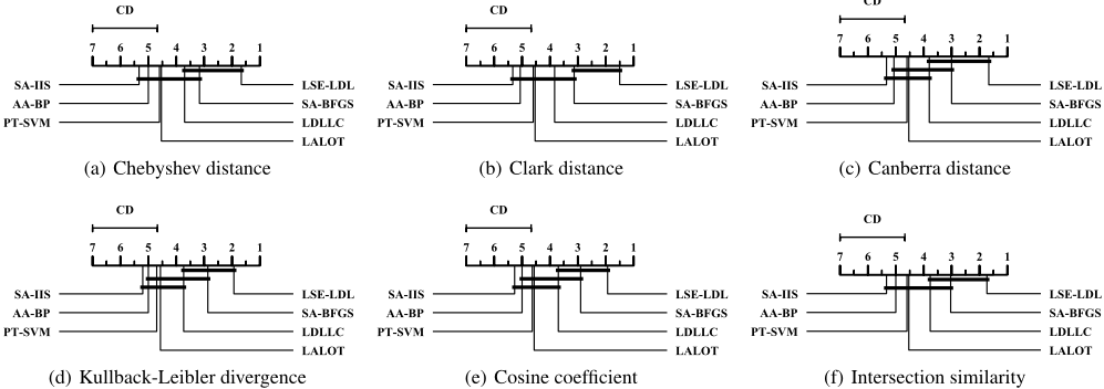
more well-founded ways, Friedman test [Friedman, 1940] is further examined which is a favorable statistical test for comparisons of more than two algorithms over multiple data sets. For each evaluation metric, Friedman test at 0.05 significance level rejects the null hypothesis of "equal" performances among all seven comparing algorithms, and then we adopt Nemenyi test to further analyze which algorithms actually differ. The performances of the two algorithms are significantly different if the corresponding average ranks over all the data sets differ by at least one critical difference (CD = 2.3254).
To visually show the actual differences of predictive performances among seven comparing LDL algorithms, the CD diagrams [Demˇsar, 2006] on each evaluation metric are illustrated in Figure 1, where the average rank of each comparing LDL algorithm is marked along the axis (higher ranks to the left). In each metric, if a group of algorithms is not significantly different under Nemenyi test, we will connect them with a thick line.
In summary, out of all 36 comparisons of predictive performances (6 baseline algorithms � 6 evaluation metrics), our LSE-LDL achieves the statistically comparable predictive performances in only 30.56% cases, and in all the other 69.44% cases, LSE-LDL achieves the statistically superior predictive performances. Besides, no algorithms have outperformed LSE-LDL. The above statistics suggest the statistical superior predictive performances of LSE-LDL as compared to all the other state-of-the-art LDL algorithms.
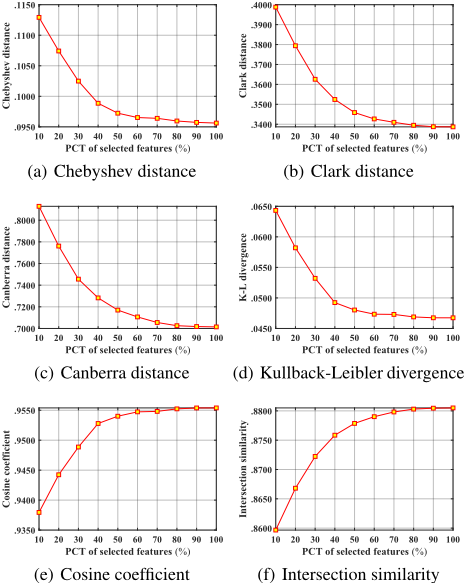
In order to examine the effectiveness of LSE-LDL in removing some irrelevant and redundant features, we also analyze the influence of the number of selected features for encoding the latent semantics. We run the testing phase of LSELDL with different Q varying from 10% to 100% of the original number of features (Stepsize: 10%). Due to space limitation, we only present the predictive performances on SJAFFE with six evaluation metrics. As shown in Figure 2, it is obvious that the performances w.r.t all six evaluation metrics tend to be stable when the percentage (PCT) of selected features is more than 60%. It means that there are 40% irrelevant and redundant features in S-JAFFE tasks, and LSE-LDL is effective in reducing storage requirements and computational overheads with superior predictive performances.
4 RelatedWork
Over the past several years, several algorithms designed for LDL have been witnessed. Generally, the existing algorithms can be grouped into the three main categories, including algorithm adaptation approaches, problem transformation approaches, and specialized approaches. Algorithm adaptation approaches directly modify some constraint conditions in traditional SLL/MLL algorithms to handle LDL tasks, such as AA-kNN [Geng et al., 2010] and AA-BP [Geng et al., 2013]. Problem transformation approaches transform the LDL task into some corresponding SLL tasks by weighted sampling on training instances, and then handle such SLL tasks through binary classifiers SVM or Naive Bayes, developing two representative problem transformation approaches, i.e., PT-SVM and PT-Bayes [Geng, 2016]. Specialized approaches focus on learning a non-linear conditional probability mass function by directly maximizing/minimizing the entropy/distance between the true and predicted label distributions. As two representative specialized approaches, both of SA-IIS and SA-BFGS [Geng et al., 2013] construct a maximum entropy model with employing Kullback-Leibler divergence as the objective function, and then implement optimization by improved iterative scaling (IIS) [Della Pietra et al., 1997] and quasi-Newton method BFGS [Nocedal and Wright, 2006], respectively. The related survey [Geng, 2016] has shown that specialized approaches are more effective than others in realworld LDL tasks, thus, more recently, researchers are all dedicated to designing highly competitive specialized approaches with considering label correlations, such as LALOT [Zhao and Zhou, 2018] and LDLLC [Jia et al., 2018].
5 Conclusion
In this paper, a novel algorithm called LSE-LDL is proposed, and it can encode the latent semantics for LDL tasks in order to alleviate the negative effects of irrelevant, redundant, and noisy features. The experimental results on 15 real-world LDL data sets validate the effectiveness of the proposed LSELDL algorithm.
Acknowledgments
This work is supported by the Natural Science Foundation of China (Nos. 61672276, 61572242), Natural Science Foundation of Jiangsu Province of China (No. BK20161406).
@inproceedings{ijcai2019p553,
  title     = {Latent Semantics Encoding for Label Distribution Learning},
  author    = {Xu, Suping and Shang, Lin and Shen, Furao},
  booktitle = {Proceedings of the Twenty-Eighth International Joint Conference on
               Artificial Intelligence, {IJCAI-19}},
  publisher = {International Joint Conferences on Artificial Intelligence Organization},
  editor    = {Sarit Kraus},
  pages     = {3982--3988},
  year      = {2019},
  month     = {8},
  note      = {Main track},
  doi       = {10.24963/ijcai.2019/553},
  url       = {https://doi.org/10.24963/ijcai.2019/553},
}
TY - CPAPER TI - Latent Semantics Encoding for Label Distribution Learning AU - Xu, Suping AU - Shang, Lin AU - Shen, Furao T2 - Proceedings of the Twenty-Eighth International Joint Conference on Artificial Intelligence, IJCAI-19 PB - International Joint Conferences on Artificial Intelligence Organization PY - 2019 SP - 3982 EP - 3988 DO - 10.24963/ijcai.2019/553 UR - https://doi.org/10.24963/ijcai.2019/553 ER -Copied
Machine-readable versions of this paper, for tools and AI agents:





