
Belief Propagation Network for Hard Inductive Semi-Supervised Learning
Proceedings of the Twenty-Eighth International Joint Conference on Artificial Intelligence. Main track. Pages 4178-4184.
https://doi.org/10.24963/ijcai.2019/580
Keywords
- Machine Learning: Classification
- Machine Learning: Semi-Supervised Learning
- Uncertainty in AI: Graphical Models
- Machine Learning: Deep Learning
Abstract
Given graph-structured data, how can we train a robust classifier in a semi-supervised setting that performs well without neighborhood information? In this work, we propose belief propagation networks (BPN), a novel approach to train a deep neural network in a hard inductive setting, where the test data are given without neighborhood information. BPN uses a differentiable classifier to compute the prior distributions of nodes, and then diffuses the priors through the graphical structure, independently from the prior computation. This separable structure improves the generalization performance of BPN for isolated test instances, compared with previous approaches that jointly use the feature and neighborhood without distinction. As a result, BPN outperforms state-of-the-art methods in four datasets with an average margin of 2.4% points in accuracy.
- [Akoglu, 2014] Leman Akoglu. Quantifying political polar- ity based on bipartite opinion networks. In ICWSM, 2014.
- [Atwood and Towsley, 2016] James Atwood and Don Towsley. Diffusion-convolutional neural networks. In NIPS, pages 1993-2001, 2016.
- [Belkin et al., 2006] Mikhail Belkin, Partha Niyogi, and Vikas Sindhwani. Manifold regularization: A geometric framework for learning from labeled and unlabeled ex- amples. Journal of Machine Learning Research, 7:2399- 2434, 2006.
- [Chau et al., 2011] Duen Horng Chau, Carey Nachenberg, Jeffrey Wilhelm, Adam Wright, and Christos Faloutsos. Polonium: Tera-scale graph mining for malware detection. In SDM, pages 131-142, 2011.
- [Chen et al., 2015] Liang-Chieh Chen, Alexander G. Schwing, Alan L. Yuille, and Raquel Urtasun. Learning deep structured models. In ICML, 2015.
- [Grover and Leskovec, 2016] Aditya Grover and Jure Leskovec. node2vec: Scalable feature learning for networks. In SIGKDD, pages 855-864, 2016.
- [Ha et al., 2012] Jiwoon Ha, Soon-Hyoung Kwon, Sang- Wook Kim, Christos Faloutsos, and Sunju Park. Top-n rec- ommendation through belief propagation. In CIKM, pages 2343-2346, 2012.
- [Hamilton et al., 2017] William L. Hamilton, Zhitao Ying, and Jure Leskovec. Inductive representation learning on large graphs. In NIPS, pages 1025-1035, 2017.
- [He and McAuley, 2016] Ruining He and Julian McAuley. Ups and downs: Modeling the visual evolution of fash- ion trends with one-class collaborative filtering. In WWW, pages 507-517, 2016.
- [Jang et al., 2016] Min-Hee Jang, Christos Faloutsos, Sang- Wook Kim, U. Kang, and Jiwoon Ha. PIN-TRUST: fast trust propagation exploiting positive, implicit, and nega- tive information. In CIKM, pages 629-638, 2016.
- [Kingma and Ba, 2015] Diederik P. Kingma and Jimmy Ba. Adam: A method for stochastic optimization. ICLR, 2015.
- [Kipf and Welling, 2017] Thomas N. Kipf and Max Welling. Semi-supervised classification with graph convolutional networks. ICLR, 2017.
- [Koller and Friedman, 2009] Daphne Koller and Nir Fried- man. Probabilistic Graphical Models -Principles and Techniques. MIT Press, 2009.
- [Li et al., 2018] Qimai Li, Zhichao Han, and Xiao-Ming Wu. Deeper insights into graph convolutional networks for semi-supervised learning. In AAAI, 2018.
- [Liang et al., 2018] Jiongqian Liang, Peter Jacobs, Jiankai Sun, and Srinivasan Parthasarathy. Semi-supervised em- bedding in attributed networks with outliers. In SDM, pages 153-161, 2018.
- [Liao et al., 2018] Renjie Liao, Marc Brockschmidt, Daniel Tarlow, Alexander L. Gaunt, Raquel Urtasun, and Richard S. Zemel. Graph partition neural networks for semi-supervised classification. In ICLR (Workshop), 2018.
- [Liao et al., 2019] Renjie Liao, Zhizhen Zhao, Raquel Urta- sun, and Richard S. Zemel. Lanczosnet: Multi-scale deep graph convolutional networks. In ICLR, 2019.
- [McAuley et al., 2015] Julian J. McAuley, Christopher Tar- gett, Qinfeng Shi, and Anton van den Hengel. Image- based recommendations on styles and substitutes. In SI- GIR, pages 43-52, 2015.
- [Ng et al., 2018] Yin Cheng Ng, Nicolò Colombo, and Ri- cardo Silva. Bayesian semi-supervised learning with graph gaussian processes. In NeurIPS, pages 1690-1701, 2018.
- [Perozzi et al., 2014] Bryan Perozzi, Rami Al-Rfou, and Steven Skiena. Deepwalk: online learning of social rep- resentations. In KDD, pages 701-710, 2014.
- [Saad, 2003] Yousef Saad. Iterative methods for sparse lin- ear systems. SIAM, 2003.
- [Sen et al., 2008] Prithviraj Sen, Galileo Namata, Mustafa Bilgic, Lise Getoor, Brian Gallagher, and Tina Eliassi- Rad. Collective classification in network data. AI Mag- azine, 29(3):93-106, 2008.
- [Srivastava et al., 2014] Nitish Srivastava, Geoffrey E. Hin- ton, Alex Krizhevsky, Ilya Sutskever, and Ruslan Salakhutdinov. Dropout: a simple way to prevent neural networks from overfitting. Journal of Machine Learning Research, 15(1):1929-1958, 2014.
- [Tamersoy et al., 2014] Acar Tamersoy, Kevin A. Roundy, and Duen Horng Chau. Guilt by association: large scale malware detection by mining file-relation graphs. In KDD, pages 1524-1533, 2014.
- [Velickovic et al., 2018] Petar Velickovic, Guillem Cucurull, Arantxa Casanova, Adriana Romero, Pietro Liò, and Yoshua Bengio. Graph attention networks. ICLR, 2018.
- [Weston et al., 2012] Jason Weston, Frédéric Ratle, Hossein Mobahi, and Ronan Collobert. Deep learning via semi- supervised embedding. In Neural Networks: Tricks of the Trade -Second Edition, pages 639-655. 2012.
- [Yang and Pedersen, 1997] Yiming Yang and Jan O. Peder- sen. A comparative study on feature selection in text cate- gorization. In ICML, pages 412-420, 1997.
- [Yang et al., 2016] Zhilin Yang, William W. Cohen, and Ruslan Salakhutdinov. Revisiting semi-supervised learn- ing with graph embeddings. In ICML, 2016.
- [Yoo et al., 2017] Jaemin Yoo, Saehan Jo, and U. Kang. Su- pervised belief propagation: Scalable supervised inference on attributed networks. In ICDM, pages 595-604, 2017.
- [Yoon et al., 2018] KiJung Yoon, Renjie Liao, Yuwen Xiong, Lisa Zhang, Ethan Fetaya, Raquel Urtasun, Richard S. Zemel, and Xaq Pitkow. Inference in prob- abilistic graphical models by graph neural networks. In ICLR (Workshop), 2018.
References were extracted automatically from the PDF and may contain errors.
Full text extracted automatically from the PDF; figures, tables and equations may differ. The PDF is the version of record.
1 Introduction
Given graph-structured data, how can we train a robust classifier in a semi-supervised setting that performs well without neighborhood information? Semi-supervised learning aims to utilize unlabeled data to improve the performance of a model. When the data are explicitly structured a graph, a typical approach to address the problem is to correlate labeled and unlabeled nodes by the graphical structure [Yang et al., 2016; Kipf and Welling, 2017; Velickovic et al., 2018].
Especially, many recent works have studied inductive approaches to develop models that perform generally well with unseen data [Hamilton et al., 2017]. Compared with transductive approaches that use the feature and neighborhood information of test data at the training time to improve the performance, such models do not use any information of the test data at the training time. As a result, they become more robust to unseen data, and their performances at the training time are easily reproduced when evaluated by unseen data.
However, recent works for inductive learning assume that every instance has enough neighborhood when input to the models, which is not true in many cases. For instance, when classifying new users in a social network who have few relationships with the others, the performance of those models is severely damaged, while being sensitive to further changes of relationships that such users generate. At the same time, it is difficult to interpret the trained relationship between features and labels since the models depend both on the feature vector and neighborhood of an instance: it is not clear which of the information mainly contributes to the performance.
In this work, we solve the hard inductive graph-based classification [Yang et al., 2016], which is to learn a classifier that works well with isolated test instances having no neighborhood information. This is essentially different from the soft inductive learning above, because it is not allowed to directly use the neighborhood information in prediction: it can help the training, but should be excluded from the final classifier. This prevents recent inductive approaches such as graph attention networks [Velickovic et al., 2018] from working well, since they use the neighborhood as essential evidence.
We propose belief propagation networks (BPN), our novel approach for training a deep neural network in a hard inductive setting. Unlike previous approaches that use features and neighborhood information together, BPN maximizes its generalization performance by separating its steps for using features and neighborhood information. First, the classification step uses an independent classifier to compute the prior distributions of nodes: it works with feature vectors and requires no neighborhood. Then, the diffusion step propagates the priors based on the message propagation [Koller and Friedman, 2009], which is used for graphical inference, and computes approximate beliefs of nodes based on the given graph.
BPN uses two kinds of loss functions on the computed beliefs. The first is a classification loss between the beliefs and observed labels, which makes the classifier work well in labeled nodes. The second is an induction loss that minimizes the difference between the priors and beliefs, which makes the classifier robust to the non-existence of neighborhood.
BPN can be coupled with any classifier because of its separable structure. For instance, a convolutional neural network (CNN) is preferred when the features represent images, or the logistic regression is useful when the relationship between features and labels should be interpreted. This makes BPN a general structure which can be used with various types of data and different objectives. BPN can also take a classifier that has been already trained and fine-tune its parameters, instead of training a new classifier from the beginning.
We conduct extensive experiments to demonstrate the superior performance of BPN, which shows the highest classifi-
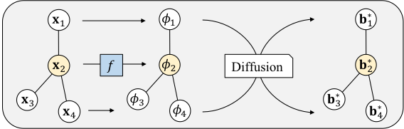
(a) Forward propagation of BPN.
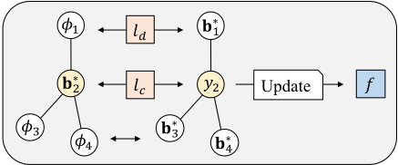
(b) Backward propagation of BPN.
Figure 1: Overview of the BPN structure. A graph of four nodes is given as an input and node 2 is the only labeled node. (a) In the forward propagation, BPN uses a classifier f to predict the priors of nodes and diffuses them to compute the beliefs. (b) In the backward propagation, BPN uses two kinds of loss functions lc and ld to use all unlabeled and labeled nodes to train a robust classifier for a hard inductive setting.
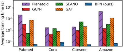
cation accuracy on four datasets compared with the state-ofthe-art approaches for inductive learning. Due to its efficient structure, training BPN is up to 150⇥ faster than training the baselines. We also show that BPN makes us interpret the relationship between features and labels, which is difficult with other approaches for soft inductive learning.
2 ProblemDefinition and RelatedWorks
We define the problem of hard inductive learning and review previous works of BPN for graph-based learning.
2.1 ProblemDefinition
We are given an undirected graph G = (V↪ E) where V and E represent the sets of nodes and edges, respectively. Each node i represents a classification instance with a feature vector xi and a label yi. All feature vectors are accessible in training, but the labels have been observed for a small subset Vo ⇢ V of the nodes. Then, we have a test set D that consists of only feature vectors, without the graphical structure. The problem of hard inductive semi-supervised classification is to train a classifier f that predicts the label of each instance x 2 D.
2.2 Transductive Learning
Transductive learning assumes that the test data are included in the graph G. Thus, a model uses their features and neighborhood information at training time and does not generalize to unseen data. Many recent approaches have been proposed for transductive learning [Atwood and Towsley, 2016; Kipf and Welling, 2017; Li et al., 2018; Yoon et al., 2018; Ng et al., 2018; Liao et al., 2018; 2019], but they are not applicable to a hard inductive setting where isolated and unseen test data are given. Previous approaches for node embedding [Grover and Leskovec, 2016; Perozzi et al., 2014] are also transductive since they generate low-dimensional representations based on the whole structure of a graph.
2.3 Inductive Learning
On the other hand, inductive learning does not use any information of test data at training [Belkin et al., 2006; Weston et al., 2012]. Planetoid [Yang et al., 2016] is an embeddingbased approach that uses the feature vectors and labels to generate representations optimized for semi-supervised learning.
In its inductive variant, the embedding is a parametric function of a feature vector and requires no neighborhood information in its prediction. To the best of our knowledge, Planetoid is the only method for hard inductive learning among recent neural network approaches, which generalizes well to isolated test instances preserving a good performance.
Other recent works focus on soft inductive learning where the test instances are given with neighborhood. GraphSAGE [Hamilton et al., 2017] generates embeddings by sampling and aggregating features from a local neighborhood. SEANO [Liang et al., 2018] is also an embedding approach but specialized for semi-supervised classification. GAT [Velickovic et al., 2018] is a neural network architecture that leverages self-attentions to address the shortcomings of graph convolutions. Compared with these approaches that jointly use features and neighborhood without distinction, BPN uses a fullyseparable structure for using these information, improving its generalization performance for hard inductive learning.
2.4 Loopy Belief Propagation
Loopy Belief Propagation (LBP) is an approximate inference algorithm that computes the posterior distributions of random variables in a graphical model [Koller and Friedman, 2009]. Due to its generality and scalability, previous works have used LBP to solve node classification problems such as large-scale malware detection [Chau et al., 2011; Tamersoy et al., 2014], social network analysis [Akoglu, 2014; Jang et al., 2016], and recommendation [Ha et al., 2012].
A recent approach [Yoo et al., 2017] has modeled LBP as a numerical function and learned the potentials by direct backpropagation from the calculated posteriors. Our work is inspired by their approach, and we use LBP to correlate nodes of a graph using an independent classifier for computing the node priors. This is effective for semi-supervised learning in a large graph, where it is difficult to estimate the potentials by a probabilistic way as in [Chen et al., 2015].
3 ProposedMethod
We propose belief propagation networks (BPN), a novel approach for hard inductive semi-supervised learning. Figure 1 depicts the overall structure of BPN. In the forward propagation, BPN first computes the prior φi of every node i using a classifier f. Then, it diffuses the priors following the graphical structure to compute the beliefs b⇤ ; this step is based on the message propagation of loopy belief propagation.
In the backward propagation of Figure 1, we use two types of loss functions to learn the classifier: the classification loss lc and induction loss ld. The classification loss lc minimizes the classification error of b⇤2 for node 2, whose label has been observed as y2. At the same time, the induction loss ld treats the beliefs as soft labels and uses the priors as predictions for the other unobserved nodes. This improves the generalization performance of f for isolated test instances.
3.1 Prediction
We describe the forward propagation of BPN in detail, which consists of two steps: prior computation and diffusion.
Prior Computation
Each node i in the given graph G represents a target instance with a feature vector xi. BPN uses an independent classifier f to estimate the prior φi of every node i:
where ✓ is a set of learnable parameters in f. This prediction is done independently from the other nodes in G, ignoring the relationships between nodes. Our main objective is to train f with a small number of observed labels so that it works well with isolated test instances in a hard inductive setting.
Probabilistic Modeling
A pairwise Markov network [Koller and Friedman, 2009] is a graphical model that represents random variables as nodes and their pairwise relationships as edges. Since the model is useful in describing properties of a real-world network, many previous works [Chau et al., 2011; Akoglu, 2014] for node classification have used it to model given networks.
We model the given graph G as a pairwise Markov network and use an edge potential matrix of size ♣S♣ ⇥ ♣S♣:
where S is the set of target states, diag(✏) is a diagonal matrix whose elements are ✏, and exp is applied elementwise to the matrix. This represents that adjacent nodes connected by an edge have the same label with a probability p proportional to exp(✏). For instance, if ♣S♣ = 3 and ✏ = 0▷1, the probability distribution of a node' state is given as (0▷32↪ 0▷36↪ 0▷32) if its neighbor has been observed as having the second label.
We call ✏ propagation strength because a property of the model is determined by the value of ✏:
- ÷ If ✏ > 0, the model induces connected nodes to have the same label because its probability is larger than the one of having different labels.
- ÷ If ✏ = 0, the nodes are considered uncorrelated and thus no information is propagated through the diffusions.
- ÷ If ✏ < 0, the nodes are negatively correlated: if a node is observed as having a certain label, then its neighbors are induced to have different labels.
The case of ✏ > 0 is the most common because most realwork networks satisfy the homophily property, which states that nearby nodes are likely to have the same label. We correlate unlabeled and labeled nodes based on the assumption of ✏ > 0, and choose its value as a hyperparameter.
Message Propagation
BPN diffuses the initial priors ⌘ times following the edges of G, maintaining two types of variables: messages and beliefs. After the t-th diffusion, a message mtij from node i to node j represents local prediction of node j estimated by node i. A belief btj is computed by aggregating the messages to node j and represents the current prediction of node j. BPN returns the beliefs ¶b⌘j ♦j2V as a result of forward propagation.
We initialize all messages and beliefs before the diffusion starts, after computing all priors:
where 1 represents a vector whose elements are all 1's. The messages are initialized as uniform distributions because the nodes have not exchanged any information at this stage. The beliefs are initialized with the predicted priors from f .
Then, the t-th messages and beliefs are computed as
where is the potential matrix, [·] represents a normalization function that divides a vector by the sum of its elements, ↵ represents the elementwise division between two vectors, and Nj represents the set of direct neighbors of node j.
The message mtij propagates the belief bt-1 i of node i to its neighbor j. Large propagation strength ✏ increases its skewness, while ✏ = 0 gives a uniform distribution as a message. The belief btj in Equation (5) aggregates the local information around node j by adding the logarithms of its prior φj and all incoming messages. As the aggregation is done at every diffusion step, the belief btj represents a predicted distribution for node j derived from its t-hop neighbors.
One important difference between BPN and previous approaches is that BPN aggregates a neighborhood's predictions with no learnable parameters. The result of diffusion is determined solely by the prediction of f . This is a main advantage since we focus on hard inductive learning, where the parameters relying on the neighborhood cannot be used at test time; BPN learns the parameters only in the classifier f.
3.2 Parameter Estimation
We learn the parameters ✓ of the classifier f by the backpropagation from the final beliefs. We propose two types of loss functions, classification loss lc and induction loss ld, for different objectives and combine them as a single loss function l which we aim to minimize.
Classification Loss
The classification loss lc measures how well the observed labels are predicted by the beliefs:
where Vo is the set of nodes whose labels have been observed, yi is the observed label of node i, and b⇤i (yi) is the predicted belief of node i for yi.
This loss function involves only a few nodes in Vo whose labels have been observed. If we use the priors, instead of the beliefs, as predicted probabilities, lc becomes a typical classification loss by f. Instead, we consider the ⌘-hop neighborhoods of Vo by using the beliefs as our predictions. Most of the nodes in G participate in lc if we use large ⌘.
However, using lc alone has two limitations. First, the performance of BPN becomes too dependent on the value of ⌘. If ⌘ is too small, many nodes remain untouched and are not used in training f. If ⌘ is too large, the training may be unstable because of a long computational chain that causes problems in gradient computations; the training will become slow, decreasing the efficiency and scalability of the algorithm. Second, BPN learns the parameters ✓ of f expecting that the priors are propagated through the graphical structure. In other words, BPN does not consider f as an independent classifier, but as a component of its structure which computes the initial beliefs. As a result, the performance of f does not generalize to the test data which have no neighborhood information and thus the diffusion has no effect. We describe how to address these limitations in the next section.
Induction Loss
We propose the induction loss ld to complement the limitations of the classification loss lc:
where S is the set of labels, and φi(s) is the prior of node i for a label s. This is the KL divergence loss between the beliefs and priors for all nodes whose labels are not given.
Minimizing ld makes the classifier f produce the priors of unobserved nodes that are as closest as possible to their beliefs. In other words, we use the priors as predictions and the beliefs as soft labels to induce f to mimic the diffusion.
The value of ld is close to zero at the first few epochs because the beliefs are distributed randomly. Then, the performance of f improves by minimizing lc, and the predicted priors on Vo are propagated to their ⌘-hop neighborhoods. This changes the beliefs of those nodes and increases the value of ld. If f is learned to decrease ld by fitting the priors to beliefs on those nodes, the new priors are propagated again to their neighborhoods, further increasing ld on the new nodes. This is repeated until all nodes are considered by ld.
Using ld overcomes the limitations of lc by the following reasons. First, BPN becomes robust to the value of ⌘ since even a small value of ⌘ is enough to correlate all nodes in G. Small ⌘ further shortens the computational chain, increasing the efficiency of gradient computation. Second, f works well on test data that have no neighborhood information, since it is trained to produce predictions that are close to the beliefs. BPN thus considers f as an independent classifier whose predictions are directly usable without further diffusions.
Overall Loss Function
We incorporate the loss functions in Equations (6) and (7) and propose the final cost function that BPN aims to minimize:
where β adjusts the balance between the two loss functions, and λ is an L2 regularization parameter for ✓. Note that BPN
Algorithm 1 Belief Propagation Network (BPN)
Require: graph G = (V↪ E), feature vectors xi for all i 2 V, and labels yi for all i 2 Vo, where Vo ⇢ V
Ensure: the trained classifier f for hard inductive learning
Require: classifier f : R♣xi♣ !R♣S♣ with parameters ✓
- 1: for [1↪ num epochs] do
- 2: b0j φj f(xj↪ ✓) for all j 2 V
- 4: for t in [1↪ ⌘] do
- 3: m0ij (1◁♣S♣)1 for all (i↪ j) 2 E
- 5: mtij [ (bt-1 i ↵mt-1 ji )] for all (i↪ j) 2 E
- 8: lc - Pi2Vo log b⌘i (yi)
- 6: btj softmax(logφj + Pi2Nj logmtij ) for all j 7: end for
- 9: ld - Pi◁2Vo Ps2S b⌘i (s)(logφi(s) - log b⌘i (s)) 10: l (1 - β)lc + βld + λ♣♣✓♣♣22 ↪
- 11: ✓ update the parameters to minimize l
- 12: end for
has no learnable parameters in its diffusion part; our target is the parameters ✓ of the classifier f. If β = 0, the induction loss is not used and f may not generalize well. If β = 1, the classification loss, which guides the induction loss in the first epochs, is not used. We thus set β in (0↪ 1).
3.3 Algorithm
We summarize BPN in Algorithm 1, which takes a classifier f as an input and trains it in a semi-supervised setting. BPN uses f to compute the priors of nodes in line 2. Then, in lines 3 to 7, BPN diffuses the priors ⌘ times to compute the final beliefs. In lines 8 to 11, BPN computes the loss l and updates the parameters ✓ of f. This is repeated until f is trained properly, and the resulting f is evaluated by test data that are not observed at training time and have no neighborhood.
Implementation
Most computations in BPN are carried out efficiently in a recent deep learning framework. However, the computation of a message mtij in Equation (4) involves a random access to the reverse direction, which is difficult for most sparse representations of adjacency matrices. The coordinate (COO) and dictionary of keys (DOK) formats support constant-time access to a random entry, but lose the spatial locality of edges, which is crucial when computing the beliefs in Equation (5). The compressed sparse row (CSR) and the compressed sparse column (CSC) formats [Saad, 2003] preserve the locality, but do not support constant access to the reverse edges.
Thus, based on the CSR format, we use an additional index array R that stores the positions of reverse edges to support constant access. As a result, the graph is represented as four arrays M, I, D, and R. Each undirected edge is stored by two directed edges inM of length 2♣E♣. I[j] contains the position of the first edge inM that is incident to node j, and D[j] has the degree of node j. For each edge in M, we set R[j] to store the position of the reverse edge of M[j] in M.
Our implementation addresses both requirements:
- ÷ Locality. If we want to compute the belief bj, all messages that go to node j are located in between M[I[j]]
| Method | Pubmed | Cora | Citeseer | Amazon |
|---|---|---|---|---|
| Planetoid | 74.6 ◦ 0.5 | 66.2 ◦ 0.9 | 66.8 ◦ 1.0 | 70.1 ◦ 1.9 |
| GCN-I | 74.1 ◦ 0.2 | 67.8 ◦ 0.6 | 63.6 ◦ 0.5 | 76.5 ◦ 0.3 |
| SEANO | 75.7 ◦ 0.4 | 64.5 ◦ 1.2 | 66.3 ◦ 0.8 | 78.6 ◦ 0.6 |
| GAT | 76.5 ◦ 0.4 | 70.1 ◦ 1.0 | 66.7 ◦ 1.0 | 77.5 ◦ 0.4 |
| BPN (ours) | 78.3 ◦ 0.3 | 72.2 ◦ 0.5 | 70.1 ◦ 0.9 | 81.5 ◦ 1.3 |
| Name | Nodes | Edges | Attributes | Labels |
|---|---|---|---|---|
| Pubmed 1 | 19,717 | 44,324 | 500 | 3 |
| Cora 1 | 2,708 | 5,278 | 1,433 | 7 |
| Citeseer 1 | 3,327 | 4,552 | 3,703 | 6 |
| Amazon | 32,966 | 63,285 | 3,000 | 3 |
and M[I[j] + D[j]] continuously.
- ÷ Reverse indexing. If we want to find the reverse of the message mij inM[k], it is located inM[R[k]].
4 Experiments
Our experiments show that BPN outperforms the state-of-theart methods for hard inductive learning.
4.1 Experimental Settings
We introduce our experimental settings including datasets, an experimental setup, and baseline methods. Our experiments are done in a workstation with Geforce GTX 1080 Ti.
Datasets
We use four datasets summarized in Table 2. The first three datasets [Sen et al., 2008] were used to evaluate the previous approaches [Velickovic et al., 2018]. The nodes represent scientific publications classified by the research areas and have feature vectors about their textual contents: TF-IDF weighted vectors in Pubmed, and bag-of-words vectors in Citeseer and Cora. The edges represent citations between the articles.
We also use an Amazon dataset based on [McAuley et al., 2015; He and McAuley, 2016]. The original dataset contains items of Amazon, each of which contains a text description, a category, and a list of related items. We use the description of each item as a bag-of-words feature vector after reducing the number of words [Yang and Pedersen, 1997]. Then, we create a network of the items by connecting related ones as edges and classify the category of each item into Electronics, Cell Phones and Accessories, or Automotive.
Experimental Setup
For each dataset, we use 20 nodes of each class for training, 1,000 nodes for testing, and 500 nodes for validation as done in [Kipf and Welling, 2017]. Since we aim to solve the hard inductive problem, we remove the neighborhood information of the test nodes to treat them as independent instances. We run every method ten times and report the average and standard deviation of classification accuracy.
1 https://github.com/kimiyoung/planetoid
We use a feedforward neural network with one hidden layer as a classifier f . Since it has a shallow structure, we use tanh as the activation function and do not use a bias. The number of hidden units is set to 32, and we use dropout [Srivastava et al., 2014] of probability 0.5. Adam [Kingma and Ba, 2015] is used as an optimizer for all datasets with different step sizes determined by validation performances.
Given the classifier f, we choose the hyperparameters of BPN based on the validation performance on Cora and use a similar setting in Citeseer: ✏ = 0▷05, λ = 10-4 , and β = 0▷9 in Cora, and ✏ is changed to 0▷01 in Citeseer. Since Pubmed and Amazon have much less labels than in Cora and Citeseer, we change the parameters to more efficient training: ✏ = 1▷0 and β = 0▷5. We lastly set λ = 2 · 10-2 in PubMed based on its small number of features. The number ⌘ of diffusion operations is set to one in all datasets, which is small but enough to correlate all nodes by the induction loss ld.
Baselines
We compare BPN with four competitive baselines recently proposed: Planetoid, GCN, GAT, and SEANO. The last two methods are considered as the state-of-the-art methods for inductive learning. We do not include GraphSAGE although it is also an inductive approach, because it focuses on either supervised or unsupervised learning: its performance on semisupervised learning has been worse than those from the other baselines [Liang et al., 2018]. We include GCN-I, an inductive variant of GCN, by removing all edges connected with the test instances. We get public implementations of the baseline methods and measure the accuracy and training time.
4.2 Classification Performance
We demonstrate that BPN outperforms the baselines by both classification accuracy and training time. Table 1 shows that BPN produces the highest accuracy with an average margin of 2.4% points, which is a significant amount considering the low standard deviations. Moreover, Figure 2 shows that BPN is trained up to 150⇥ faster than the recent baselines, which consider multi-hop neighbors of each instance with extensive amounts of computations. These are due to the efficient structure of BPN that considers only a small number of neighbors at each epoch but eventually correlates all labeled and unlabeled nodes by minimizing two kinds of loss functions.
4.3 Interpretability
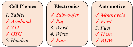
Since the prediction of the previous approaches relies both on the feature and neighborhood information of an instance, it is difficult to interpret the resulting models. On the other hand, the learned classifier f from BPN uses only the features, and it is possible to analyze the relationship between the features and labels. One way to interpret f is to give a zero input and differentiate the prediction with regard to the input. Then, the gradient of each element represents its importance for classification. Figure 5 shows the top five keywords of the largest importances for each class on Amazon, each of which corresponds to an element of the bag-of-words vectors. Although the checked words are not present in the labeled nodes, we note that they are learned successfully by BPN and used to predict the test instances by f as important evidence.
4.4 Effects of the Losses
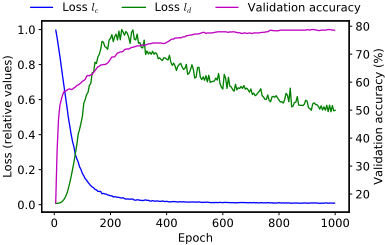
BPN minimizes two kinds of loss functions to perform well in a hard inductive setting. Figure 3 shows their values during the training of BPN on Cora. At first, the classification loss lc is at maximum, while the induction loss ld is the smallest since most priors and beliefs are close to uniform distributions and thus similar to each other. BPN then minimizes lc on the labeled nodes, changing the beliefs of their neighborhoods by diffusion; this increases ld instead. After that, BPN moves to the unlabeled nodes and updates its parameters to produce priors that are as closest as possible to their beliefs, minimizing ld in latter epochs. The validation accuracy keeps increasing whether we focus on lc or ld.
4.5 Hyperparameter Study
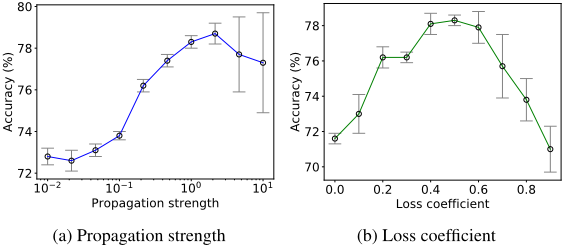
We conduct various experiments on BPN to see the effect of each hyperparameter on its performance. The results for two hyperparameters ✏ and β are summarized in Figure 4. Larger ✏ leads to higher accuracy until a certain point, and then the deviation sharply increases, decreasing the average accuracy. This is because large ✏ propagates more information at each diffusion, decreasing the stability. In terms of the loss coefficient, β = 0▷5 gives the best balance between the two losses. It is notable that larger deviations are observed when β > 0▷5, since in that case ld starts to be minimized before f is fully optimized for the labeled nodes by minimizing lc.
5 Conclusion
In this work, we have proposed belief propagation networks (BPN), a novel approach for hard inductive semi-supervised learning. BPN takes a differentiable classifier as an input and trains it efficiently by minimizing two types of loss functions, improving both its classification performance and robustness to the non-existence of neighborhood. As a result, the trained classifier outperforms the state-of-the-art approaches in four datasets for text classification. Moreover, the separable structure of BPN makes the classifier interpretable in terms of the relationship between features and labels, which is difficult in previous approaches for soft inductive learning. Future works include designing an improved message passing operation for heterogeneous or edge-attributed networks.
Acknowledgments
This work was supported by the ICT R&D program of MSIT/IITP (No.2017-0-01772 , Development of QA systems for Video Story Understanding to pass the Video Turing Test). The Institute of Engineering Research at Seoul National University provided research facilities for this work. The ICT at Seoul National University provides research facilities for this study. U Kang is the corresponding author.
@inproceedings{ijcai2019p580,
  title     = {Belief Propagation Network for Hard Inductive Semi-Supervised Learning},
  author    = {Yoo, Jaemin and Jeon, Hyunsik and Kang, U},
  booktitle = {Proceedings of the Twenty-Eighth International Joint Conference on
               Artificial Intelligence, {IJCAI-19}},
  publisher = {International Joint Conferences on Artificial Intelligence Organization},
  editor    = {Sarit Kraus},
  pages     = {4178--4184},
  year      = {2019},
  month     = {8},
  note      = {Main track},
  doi       = {10.24963/ijcai.2019/580},
  url       = {https://doi.org/10.24963/ijcai.2019/580},
}
TY - CPAPER TI - Belief Propagation Network for Hard Inductive Semi-Supervised Learning AU - Yoo, Jaemin AU - Jeon, Hyunsik AU - Kang, U T2 - Proceedings of the Twenty-Eighth International Joint Conference on Artificial Intelligence, IJCAI-19 PB - International Joint Conferences on Artificial Intelligence Organization PY - 2019 SP - 4178 EP - 4184 DO - 10.24963/ijcai.2019/580 UR - https://doi.org/10.24963/ijcai.2019/580 ER -Copied
Machine-readable versions of this paper, for tools and AI agents:





