
Light-Weight Hybrid Convolutional Network for Liver Tumor Segmentation
Proceedings of the Twenty-Eighth International Joint Conference on Artificial Intelligence. Main track. Pages 4271-4277.
https://doi.org/10.24963/ijcai.2019/593
Keywords
- Computer Vision: Biomedical Image Understanding
- Computer Vision: 2D and 3D Computer Vision
- Machine Learning: Deep Learning
Abstract
Automated segmentation of liver tumors in contrast-enhanced abdominal computed tomography (CT) scans is essential in assisting medical professionals to evaluate tumor development and make fast therapeutic schedule. Although deep convolutional neural networks (DCNNs) have contributed many breakthroughs in image segmentation, this task remains challenging, since 2D DCNNs are incapable of exploring the inter-slice information and 3D DCNNs are too complex to be trained with the available small dataset. In this paper, we propose the light-weight hybrid convolutional network (LW-HCN) to segment the liver and its tumors in CT volumes. Instead of combining a 2D and a 3D networks for coarse-to-fine segmentation, LW-HCN has a encoder-decoder structure, in which 2D convolutions used at the bottom of the encoder decreases the complexity and 3D convolutions used in other layers explore both spatial and temporal information. To further reduce the complexity, we design the depthwise and spatiotemporal separate (DSTS) factorization for 3D convolutions, which not only reduces parameters dramatically but also improves the performance. We evaluated the proposed LW-HCN model against several recent methods on the LiTS and 3D-IRCADb datasets and achieved, respectively, the Dice per case of 73.0% and 94.1% for tumor segmentation, setting a new state of the art.
- [Akinyemiju et al., 2017] Tomi Akinyemiju, Semaw Abera, et al. The burden of primary liver cancer and underlying etiologies from 1990 to 2015 at the global, regional, and national level: results from the global burden of disease study 2015. JAMA oncology, 3(12):1683-1691, 2017.
- [Carreira and Zisserman, 2017] Joao Carreira and Andrew Zisserman. Quo vadis, action recognition? a new model and the kinetics dataset. In CVPR, pages 4724-4733, 2017.
- [Chen et al., 2016] Tianqi Chen, Bing Xu, Chiyuan Zhang, and Carlos Guestrin. Training deep nets with sublinear memory cost. arXiv preprint arXiv:1604.06174, 2016.
- [Chen et al., 2018a] Liang-Chieh Chen, George Papandreou, Iasonas Kokkinos, Kevin Murphy, and Alan L Yuille. Deeplab: Semantic image segmentation with deep convo- lutional nets, atrous convolution, and fully connected crfs. IEEE-TPAMI, 40(4):834-848, 2018.
- [Chen et al., 2018b] Liang-Chieh Chen, Yukun Zhu, George Papandreou, Florian Schroff, and Hartwig Adam. Encoder-decoder with atrous separable convolution for se- mantic image segmentation. In ECCV, pages 801-818, 2018.
- [Chlebus et al., 2017] Grzegorz Chlebus, Hans Meine, Jan Hendrik Moltz, and Andrea Schenk. Neural network-based automatic liver tumor segmentation with random forest-based candidate filtering. arXiv preprint arXiv:1706.00842, 2017.
- [Chlebus et al., 2018] Grzegorz Chlebus, Andrea Schenk, Jan Hendrik Moltz, Bram van Ginneken, Horst Karl Hahn, and Hans Meine. Automatic liver tumor segmentation in ct with fully convolutional neural networks and object-based postprocessing. Scientific reports, 8(1):15497, 2018.
- [Chollet, 2017] Francois Chollet. Xception: Deep learning with depthwise separable convolutions. In CVPR, pages 1251-1258, 2017.
- [Dou et al., 2017] Qi Dou, Lequan Yu, Hao Chen, Yueming Jin, Xin Yang, Jing Qin, and Pheng-Ann Heng. 3D deeply supervised network for automated segmentation of volu- metric medical images. Medical Image Analysis, 41:40- 54, 2017.
- [Foruzan and Chen, 2016] Amir Hossein Foruzan and Yen- Wei Chen. Improved segmentation of low-contrast lesions using sigmoid edge model. International Journal of Com- puter Assisted Radiology and Surgery, 11(7):1267-1283, 2016.
- [Han, 2017] Xiao Han. Automatic liver lesion segmentation using a deep convolutional neural network method. arXiv preprint arXiv:1704.07239, 2017.
- [Kingma and Ba, 2015] Diederik P. Kingma and Jimmy Lei Ba. Adam: a method for stochastic optimization. In ICLR, pages 1-15, 2015.
- [Li et al., 2018a] Xiaomeng Li, Hao Chen, Xiaojuan Qi, Qi Dou, Chi-Wing Fu, and Pheng-Ann Heng. H- denseunet: Hybrid densely connected unet for liver and tumor segmentation from CT volumes. IEEE-TMI, 37(12):2663-2674, 2018.
- [Li et al., 2018b] Xiaomeng Li, Qi Dou, Hao Chen, Chi- Wing Fu, Xiaojuan Qi, Daniel L Belavỳ, Gabriele Arm- brecht, Dieter Felsenberg, Guoyan Zheng, and Pheng-Ann Heng. 3D multi-scale FCN with random modality voxel dropout learning for intervertebral disc localization and segmentation from multi-modality MR images. Medical Image Analysis, 45:41-54, 2018.
- [Long et al., 2015] Jonathan Long, Evan Shelhamer, and Trevor Darrell. Fully convolutional networks for seman- tic segmentation. In CVPR, pages 3431-3440, 2015.
- [Moghbel et al., 2016] Mehrdad Moghbel, Syamsiah Mashohor, Rozi Mahmud, and M Iqbal Bin Saripan. Automatic liver segmentation on computed tomography using random walkers for treatment planning. EXCLI journal, 15:500, 2016.
- [Qiu et al., 2017] Zhaofan Qiu, Ting Yao, and Tao Mei. Learning spatio-temporal representation with pseudo-3D residual networks. In ICCV, pages 5534-5542, 2017.
- [Ronneberger et al., 2015] Olaf Ronneberger, Philipp Fis- cher, and Thomas Brox. U-net: Convolutional networks for biomedical image segmentation. In MICCAI, pages 234-241, 2015.
- [Tran et al., 2015] Du Tran, Lubomir Bourdev, Rob Fergus, Lorenzo Torresani, and Manohar Paluri. Learning spa- tiotemporal features with 3D convolutional networks. In ICCV, pages 4489-4497, 2015.
- [Tran et al., 2018] Du Tran, Heng Wang, Lorenzo Torresani, Jamie Ray, Yann LeCun, and Manohar Paluri. A closer look at spatiotemporal convolutions for action recognition. In CVPR, pages 6450-6459, 2018.
- [Vorontsov et al., 2018] Eugene Vorontsov, An Tang, Chris Pal, and Samuel Kadoury. Liver lesion segmentation in- formed by joint liver segmentation. In ISBI, pages 1332- 1335, 2018.
- [Wu et al., 2017] Weiwei Wu, Shuicai Wu, Zhuhuang Zhou, Rui Zhang, and Yanhua Zhang. 3D liver tumor segmentation in CT images using improved fuzzy C- means and graph cuts. BioMed Research International, 2017(5207685):1-11, 2017.
- [Xie et al., 2018] Saining Xie, Chen Sun, Jonathan Huang, Zhuowen Tu, and Kevin Murphy. Rethinking spatiotem- poral feature learning: Speed-accuracy trade-offs in video classification. In ECCV, pages 305-321, 2018.
- [Yu and Koltun, 2016] Fisher Yu and Vladlen Koltun. Multi- scale context aggregation by dilated convolutions. In ICLR, pages 1-13, 2016.
- [Yu et al., 2017] Lequan Yu, Hao Chen, Qi Dou, Jing Qin, and Pheng-Ann Heng. Automated melanoma recognition in dermoscopy images via very deep residual networks. IEEE-TMI, 36(4):994-1004, 2017.
- [Zhao et al., 2017] Hengshuang Zhao, Jianping Shi, Xiao- juan Qi, Xiaogang Wang, and Jiaya Jia. Pyramid scene parsing network. In CVPR, pages 2881-2890, 2017.
References were extracted automatically from the PDF and may contain errors.
Full text extracted automatically from the PDF; figures, tables and equations may differ. The PDF is the version of record.
1 Introduction
The liver is a common site of tumor development, which causes massive deaths every year [Akinyemiju et al., 2017]. Liver tumor segmentation, a fundamental step in the computer-aided diagnosis, aims to segment tumors in contrast-enhanced abdominal computed tomography (CT) volumes. A reliable liver tumor segmentation system is able to assist doctors in the accurate evaluation of primary or secondary tumor development and fast therapeutic schedule. Automated segmentation of tumors in the liver is, however, challenging due to three issues: (1) the low contrast between tumors and liver or other organs in CT volumes, (2) the heterogeneity of liver tumors in shape, size, number, and location, and (3) inadequate training data with pixel-level annotation.
Recently, deep convolutional neural networks (DCNNs) have led to significant breakthroughs in image segmentation [Long et al., 2015]. Following this trend, many attempts have been made to extend these successes to liver tumor segmentation [Li et al., 2018a]. Generally, the DCNNs designed for image segmentation can be divided into two categories: 2D and 3D networks. 2D DCNNs have achieved good performance in many 2D scenarios of medical image segmentation [Yu et al., 2017], as they have done in natural image segmentation [Chen et al., 2018b]. However, these 2D networks can only be applied to 2D slices without exploring the inter-slice correlations, and hence are not good segmentation tools for volumetric liver tumors. Let us make an analogy between an abdominal CT volume and a video. A volumetric liver tumor segmentation algorithm must be able to explore both the spatial (i.e. intra-slice) and temporal (i.e. inter-slice) information simultaneously. To address this issue, 3D DCNNs have been constructed, which, unfortunately, have an excessive number of parameters and extremely high complexity. Therefore, it is difficult to train a 3D DCNN with limited training data and hardware resources. Besides, 3D DCNNs requires much more time in the inference than 2D DCNNs, which is against the fast clinical diagnosis.
To balance between the model complexity and segmentation accuracy, hybrid models, which replace some 3D convolutions in 3D DCNNs with 2D convolutions, have been proposed and have shown their effectiveness in video classification [Xie et al., 2018; Tran et al., 2018]. Although partly reducing the complexity, this kind of hybrid models still have a mass number of parameters caused by the rest of 3D convolutions and still require large scale datasets for training. A popular solution that leads to a significantly enhanced performance in video analysis is transfer learning, i.e. pre-training a network on large scale datasets, like Sports-1M and Kinetics, and fine-tuning it on small datasets. However, due to the cost related to abdominal CT data acquisition and annotation, there is no large scale dataset for liver tumor segmentation. The data limitation definitely hinders the success of 3D DCNNs and hybrid models. Hence, reducing the computational complexity and number of parameters is indispensable when training a DCNN for liver tumor segmentation.
In this paper, we propose the light-weight hybrid convolutional network (LW-HCN) to segment liver tumors in contrast-enhanced abdominal CT volumes. The LW-HCN model has a 3D encoder-decoder structure but with only 3.6 million parameters. To achieve this, we replace the 3D convolutions at the bottom of the encoder with low-cost 2D convolutions, concatenate the obtained 2D feature maps into a 3D feature map, feed it to 3D convolutions to capture highlevel semantic information in both spatial and temporal dimensions, and then use a simple 3D decoder to recover the spatial and temporal information for the output. Comparing with other hybrid models, our model is unique in two aspects. First, we jointly use 2D and 3D convolutions in the same network, instead of using a 2D network for coarse segmentation and a 3D network for refinement. Second, we design the depthwise and spatiotemporal separate (DSTS) factorization for 3D convolutions, which drastically reduces model parameters and the computational cost while improving performance. We evaluated the LW-HCN model against the stateof-the-art methods on the LiTS dataset and the 3D-IRCADb dataset. The main contributions are summarized as follows:
- We propose the LW-HCN model that jointly uses both 2D and 3D convolutions for effective and efficient segmentation of liver tumors in CT volumes.
- We design the DSTS factorization for 3D convolutions, which not only reduces model parameters drastically but also improves the performance.
- The proposed LW-HCN model has merely 3.6 million parameters (only 15.3 MB) but achieved the state-of-theart performance on the LiTS and 3D-IRCADb datasets.
2 RelatedWork
2.1 2DDCNNModels
DCNN models based on 2D convolutions have achieved the state-of-the-art performance on many image segmentation benchmarks. The significant performance improvement is mainly attributed to many newly designed architectures, including the spatial pyramid pooling [Zhao et al., 2017; Chen et al., 2018a] for exploiting the multi-scale information, the atrous convolution [Yu and Koltun, 2016] for expanding the receptive field, and the skip connection [Ronneberger et al., 2015] for capturing the detailed information by reusing low-level but high-resolution feature maps. Inspired by these breakthroughs, research efforts have been devoted to the leverage of 2D convolutional networks for liver tumor segmentation. [Vorontsov et al., 2018] connect two UNet-like fully convolutional networks in tandem and train them end-to-end for the joint segmentation of the liver and tumors. [Han, 2017] proposes a 2D residual UNet model which takes a stack of adjacent slices as input and produces the segmentation map corresponding to the center slice. A common weakness of these 2D models is the lack of capturing the temporal information of liver tumors, which may degrade the performance in volumetric segmentations.
2.2 3DDCNNModels
3D convolutions are able to simultaneously explore the temporal and spatial information, and hence are extremely useful in 3D scenarios. [Tran et al., 2015] adopt a 3D DCNN
(C3D) for the spatiotemporal feature learning in video classification. [Carreira and Zisserman, 2017] propose an 3D inception model which inflates the filters and pooling kernels of 2D Inception V1 model into 3D convolutions and bootstraps parameters by repeating the weights of 2D filters along the temporal dimension. To reduce the parameters of 3D convolutions, [Qiu et al., 2017] split the standard 3D convolution into a spatial-wise convolution and a temporal-wise convolution. This kind of decomposition strategy has been used in a variety of works, including the S3D [Xie et al., 2018] and R(2+1)D [Tran et al., 2018] models.
Based on the strong spatiotemporal feature learning ability of 3D convolutions, [Dou et al., 2017] present a 3D fully convolutional network to generate high-quality score maps for automated liver segmentation. [Li et al., 2018b] introduce a multi-scale context mechanism in 3D networks to harness multi-scale contextual information for intervertebral discs segmentation. As expected, 3D convolutions show a better ability to capture both spatial and temporal information. However, 3D DCNNs have more parameters and need more computation than their 2D counterparts. It means that, for a 3D DCNN, achieving a good performance relies extremely on powerful computation devices and large scale datasets. Unfortunately, the insufficiency of training samples limits the success of 3D DCNNs in the liver tumor segmentation, which is a small-sample learning problem.
2.3 Hybrid Architectures
Recently, hybrid architectures, which jointly use 2D and 3D convolutions to reduce the model complexity, have been proposed and successfully applied to video classification. [Tran et al., 2018] propose to use 3D convolutions in either the bottom or top layers and 2D convolutions in other layers. [Xie et al., 2018] replace 3D convolutions at the bottom of the model which contributes to the best performance in both speed and accuracy. Similarly, both hybrid models factorize a standard 3D convolution into a spatial convolution followed by a temporal convolution, and thus extremely reduces the parameters of 3D convolutions. Different from these methods, our LWHCN model drastically reduces the computational complexity by applying the depthwise operation to both 2D and 3D convolutions. Besides, we introduce an efficient 3D convolution factorization to separate the temporal feature learning from the spatial feature learning in a parallel mode.
For the liver tumor segmentation, [Li et al., 2018a] propose a hybrid densely connected UNet model which is composed of a 2D segmentation network and a 3D segmentation network. The 2D network is used to extract image-level features and perform segmentation on a slice-by-slice basis. The pixel-wise probabilities produced by the 2D network are then concatenated with the original 3D volume and fed into the 3D network for a refinement. Different from it, we only use one network which consists of both 2D and 3D convolutions and effectively reduce the model complexity by factorizing the high-cost 3D convolutions.
3 Approach
Fig. 1 illustrates the overview of our LW-HCN model. In this section we first elaborate the proposed DSTS factoriza- D convolutions
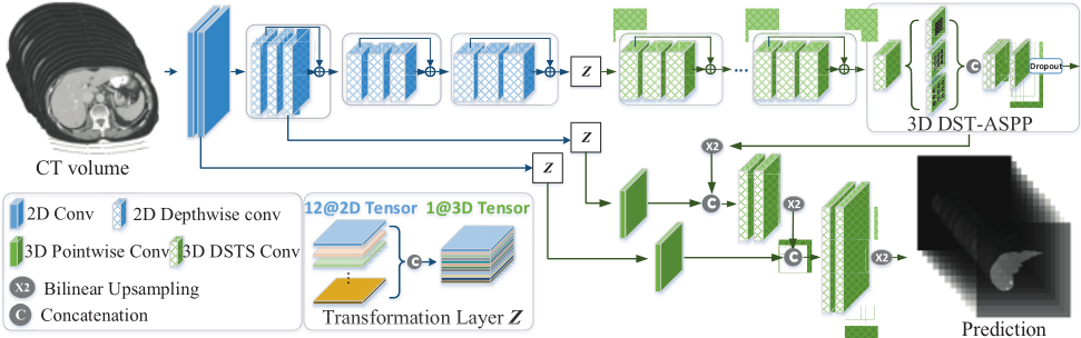
... tion for 3D convolutions which capture both spatial and temporal information with low computation complexity. Then, we develop a novel LW-HCN model with an encoder-decoder structure, which is composed of 2D depthwise convolutions in the bottom and 3D DSTS convolutions in the rest. Besides, we also apply several parallel 3D atrous DSTS convolutions with different rates (called depthwise and spatiotemporal atrous spatial pyramid pooling, DST-ASPP) at the end of the encoder to capture multi-scale information.
3.1 DSTS Factorization for 3DConvolutions
Depthwise Convolution for 3D: The depthwise convolution, usually followed by a pointwise convolution, reduces the computation and parameters by performing convolutions for each input channel independently. 2D depthwise convolution has been successfully used in [Chollet, 2017]. In this work, we extend the depthwise convolution to 3D.
Let us consider a 3D convolution layer that takes a TF × WF ×HF ×M feature map F as input and produces a TG × WG × HG × N feature map G as output, where T∗, W∗, H∗ are temporal dimension, spatial width, and spatial height of 3D feature maps, respectively, and M and N are the number of input and output channels, respectively. We parameterize a standard 3D convolution layer through a X × Y × Z × M ×N convolution kernel KS , where X, Y , Z are temporal and spatial dimension of the kernel. The output of this 3D convolution layer can be computed as
where r represents the r-dilated convolution operation. As for a 3D depthwise convolution layer with a X ×Y ×Z ×M kernel KD , the mathematical formulation is as follow:
(2) After that, we apply a 3D pointwise convolution with 1×1× 1 ×M ×N kernel KP to combine the output of depthwise convolution and project it into a new channel space as follows
D Depthwise Separate Conv D Depthwise and Spatiotemporal Separate Conv Bilinear Upsampling Concatenation Element wise Add The depthwise convolution is a powerful operation to reduce convolution parameters and computational complexity. Let's consider a 3×3×3 convolution operation with the input channel c and output channel c. A standard 3 × 3 × 3 convolution contains 27c2 parameters and a depthwise convolution only has 27c parameters which is decreased by a factor of c.
Dropou t D DST ASPP D convolutions DST ASPP ... Spatiotemporal Separate Convolution: 3D convolutions have more parameters and require more computations than 2D convolutions. To get a light-weight model, a straightforward solution is to factorize a standard 3D convolution into two separate convolutions, i.e., a 1×Y ×Z spatial convolution and a X × 1 × 1 temporal convolution, which are defined as the spatiotemporal separate (STS) convolution. The spatial convolution focus on the spatial feature learning, while the temporal convolution focus on the temporal feature learning. We introduce two kinds of STS convolution modules, i.e., a sequential STS module and a parallel STS module, which are defined as follows:
where KS1 represents the kernel of the 1 × Y × Z spatial convolution, KS2 represents the kernel of the X×1×1 temporal convolution, and ∪ denotes the concatenation of feature maps. Both STS modules separate temporal and spatial convolutions, and hence reduce the parameters of a standard 3 × 3 × 3 convolution from 27c2 to 12c2 .
In the sequential STS module, the spatial and temporal convolutions are performed in sequence, i.e. using the output of spatial convolution as the input of temporal convolution. In the parallel STS module, these two convolutions are performed in parallel in two branches, and their outputs are then concatenated. Compared with the sequential module, the parallel one better separates the temporal feature learning from spatial feature learning. Considering the anisotropic spatial resolution of abdominal CT volumes, we adopt the parallel STS module for 3D liver tumor segmentation, which shows better performance than the sequential module in Section 4.3.
3D DSTS Convolution: To further reduce the computational complexity and model parameters, we propose the 3D DSTS convolution. As shown in Fig. 2, we divide the output channels of the previous layer into a spatial branch and a temporal branch, which focus on the spatial and temporal feature Concat
...
Temporal branch Previous Layer
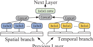
Figure 2: Diagram of the 3D DSTS convolution module.
learning, respectively. In each branch, the spatial / temporal convolution is carried out in each channel. After the separate feature learning, the outputs of spatial and temporal branches are concatenated and fed to a pointwise convolution for feature integration. The formulation of 3D DSTS convolution is
where KP is the kernel of pointwise convolution, KD1 and KD2 are kernels of spatial and temporal convolutions, respectively. We replace all 3D convolutions with the DSTS convolutions, which dramatically reduces the number of parameters from 27c2 to c2 + 12c for each convolution operation.
3.2 Hybrid Convolutional Network
Dimension Transformation Layer: To bridge the 2D and 3D convolutions, we introduce a transformation layer Z, which is used to transform 2D feature maps into 3D maps. In Fig. 1, we first use 2D convolutions to extract feature maps from 2D slices in the same CT volume, and then concatenate them into a 3D feature map along the temporal dimension.
DST-ASPP: The size of liver tumors varies greatly, ranging from as small as dozens of voxels to extremely big ones. To effectively capture the multi-scale information, we propose the following 3D DST-ASPP module and apply it to the top output of the encoder
where ⋃ represents the concatenation of feature maps, and Q is the number of DSTS convolution modules. Inspired by the 2D ASPP used in [Chen et al., 2018b], we perform a 1 × 1 × 1 convolution, and three DSTS convolutions with the atrous rates 2, 4, 6 in the spatial dimension. The obtained feature maps are concatenated and passed through a pointwise convolution layer. Different from [Chen et al., 2018b], we perform a 3D module and replace all standard 3D convolutions with the DSTS convolutions which separate temporal convolutions from spatial ones and drastically reduce the computational complexity.
Encoder-Decoder Architecture: The proposed LW-HCN model has an encoder-decoder architecture. The encoder part contains a series of 2D convolutions and 3D convolutions. We adopt 2D depthwise convolutions at the bottom of the encoder to gradually reduce the feature maps resolution by a factor of 8, and then transform the 2D feature maps into 3D ones through the transformation layer Z. Next, we apply the 3D DSTS convolutions to capture spatial and temporal semantic information. At the end of encoder, we apply the 3D DST-ASPP to capture multi-scale information. After that, a dropout layer with a rate of 0.5 is added to avoid overfitting. In the decoder, the bilinear upsampling is used to recover the resolution of feature maps in spatial dimension. The upsampled feature maps are concatenated with the low-level but high-resolution features, which are transformed from the outputs of the bottom 2D convolutions, and passed through 3D DSTS convolutions for feature refinements. Finally, the 3D predictions are transformed to 2D results which correspond to the input.
Loss Function: The 3D liver tumor segmentation suffers from the extreme class-imbalance. The proportion of tumors accounts for only one hundredth, even one thousandth of nontumor regions in each CT volume. To address this issue, we jointly use the multi-class Dice loss, which is less sensitive to class imbalance, and the cross entropy (CE) loss. The combined loss can be calculated as follows
where C denotes the number of categories, V denotes the number of voxels, pci represents the predicted probability of voxel i belonging to the class c, yc i represents the ground truth label of voxel i, and ε is a smooth factor.
4 Experiments
4.1 Dataset
We evaluated the LW-HCN model on the LiTS dataset and 3D-IRCADb dataset. The LiTS dataset is composed of 201 contrast-enhanced abdominal CT volumes provided by various clinical sites around the world, including 131 volumes for training and 70 volumes for testing. The pixel-wise segmentation ground truths of the liver and tumors in training set are publicly available, but the ground truths for test cases are withheld for online validation. The 3D-IRCADb dataset offers 20 venous phase enhanced CT volumes acquired from various European hospitals with different CT scanners. These CT volumes are composed of dozens to about one thousand slices of size 512 × 512. Different from natural images, the voxel value in a CT volume is the Hounsfield Unit (HU) value with a range from -1000 (air at standard pressure and temperature) to more than +3000 (dense bone). To remove irrelevant information, we truncate the HU values of all volumes to the range [-200,+250] as done in [Li et al., 2018a], and then normalized them linearly to [-1, +1].
Following the evaluation procedures of the LiTS challenge 1 , we evaluated the segmentation performance with a global Dice score (Dice global), i.e., combining all data sets into one, and an average of Dice per volume score (Dice per case). Dice per case is the only golden indicator, according to which all methods are ranked. We also adopted the root mean square error (RMSE) to assess the tumor burden.
4.2 Implementation Details
Our model is implemented with Keras and optimized with the Adam algorithm [Kingma and Ba, 2015] on a NVIDIA Tesla P100 GPU. The parameters of 2D convolutions are initialized using the DeepLabV3+ model [Chen et al., 2018b] which is pre-trained on the MS-COCO and PASCAL VOC datasets and fine-tuned on the LiTS dataset, while the 3D convolutional layers are trained from scratch. The initial learning rate is set to 0.001 and decayed according to the poly schedule lr = lr × (1 - iterations/total iterations)0.9 . We select 5 volumes from the LiTS training data to form a validation set, which is used to monitor the performance of our model. During training, we densely sample 12 × 256 × 256 sub-volumes from each CT scan as the input of the model. To save the GPU memory, we adopt the gradient-checkpointing algorithm [Chen et al., 2016] to enlarge the batch size to 6. Based on the fully convolutional architecture, our LW-HCN model can accept an input with an arbitrary size in the test stage. We extract the sub-volumes from each test CT volume every 10 slices. Each sub-volume consists of 20 sequential slices with a full size of 512 × 512. The final prediction for a whole volume is generated by combing and averaging the scores of these sub-volumes. In our experiments, it takes about 24 hours to train the LW-HCN model and costs only 10 to 80 seconds to segment each test volume, depending on the number of slices. To evaluate the generalization ability of the LW-HCN model, we apply directly the model trained on the LiTS Challenge dataset to the 3D-IRCADb dataset.
1 https://competitions.codalab.org/competitions/17094#learn the details
| Factorization | #Params (×106 ) | Size (MB) | Time (ms) | Dice per case (tumor/liver,%) |
|---|---|---|---|---|
| standard 3D | 38.6 | 154.7 | 708.1 | 65.4/97.1 |
| STS(sequ) | 19.4 | 78.1 | 566.1 | 66.0/97.0 |
| STS(pa) | 20.8 | 84.1 | 597.5 | 67.3/97.0 |
| DSTS | 3.6 | 15.3 | 404.8 | 69.7/97.4 |
| Models | Tumor | Liver |
|---|---|---|
| LW-HCN+Ldice | 65.7 | 96.4 |
| LW-HCN+ASPP+Ldice | 66.8 | 96.9 |
| LW-HCN+ASPP+Skip+Ldice | 68.5 | 97.3 |
| LW-HCN+ASPP+Skip+Ldice+Lce | 69.7 | 97.4 |
4.3 Ablation Study
Depthwise and Spatiotemporal Factorization: We compared the proposed LW-HCN model that uses DSTS convolutions to its variants that uses either the sequential or parallel STS convolutions and the baseline that uses standard 3D convolutions on 5 validation volumes (V1-V5). Tab. 1 gives the number of parameters, size, inference time (based on a single input with 12 slices of spatial size 512 × 512), and the segmentation accuracy of each model. The baseline model has 38.6 million parameters, a size of 154.7 MB, and inference time of about 700 ms, and achieved a Dice per case of 65.4% and 97.1% for tumor and liver segmentation, respectively. Comparing with the baseline, both variant models have less parameters, a smaller size, and less inference time, but a higher accuracy in tumor segmentation. Furthermore, it shows that the parallel STS results in more accurate tumor segmentation than the sequential STS, though it has slightly more parameters, larger size, and higher inference time. With the proposed DSTS convolutions, our LW-HCN model has only 3.6 million parameters and 15.3 MB in size, which are almost one tenth of those of the baseline model. However, comparing with both the baseline and other two factorizations, it not only improves the accuracy of liver segmentation slightly, but also improves the accuracy of tumor segmentation (i.e. from 67.3% to 69.7%) and reduces the inference time substantially.
Tab. 2 gives the Dice per case obtained by applying our LW-HCN model with different settings to the LiTS validation set. Three conclusions can be drawn from this table. DST-ASPP: Motivated by the effectiveness of spatial pyramid pooling, we introduce a 3D DST-ASPP to capture the multiscale information in CT volumes, which brings 1.1% and 0.5% increase of the Dice per case for tumor and liver segmentation, respectively. 2D-3D skip connections: We adopt the 2D-3D skip connections to transform the low-level but high-resolution 2D features to 3D features and feed them into the high-level decoder, which leads to 1.7% and 0.4% improvements of the Dice per case for tumor and liver segmentation, respectively. Loss function: To optimize the LW-HCN model efficiently, we replace the Dice loss with our combined loss, which further improves Dice per case by 1.2% and 0.1% for tumor and liver segmentation, respectively.
4.4 Comparative Experiments
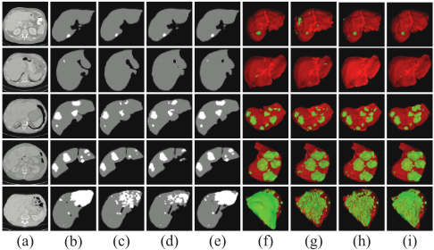
Tab. 3 shows the performance of the proposed LW-HCN model and state-of-the-art 2D, 3D and hybrid models on the LiTS test set. Fig. 3 shows a typical 2D slice extracted from each of five validation volumes, ground truth, segmentation results obtained by DeeplabV3+ [Chen et al., 2018b], I3D [Carreira and Zisserman, 2017], and our LW-HCN model, respectively, and the corresponding 3D visualization. It shows that our LW-HCN model performs better than other models in the segmentation of small tumors (see 1st and 2nd volumes) and smoothing the surface of big tumors, due to an improved ability to learn both spatial and temporal features.
Comparing with 2D Models: Due to the lack of the ability to learn temporal features, 2D models, including ResUNet, TwoFCNs [Vorontsov et al., 2018], DeeplabV3+, 2.5D ResUNet [Han, 2017], and UNet+SP [Chlebus et al., 2018], under-perform the LW-HCN model, which shows a strong ability to learn both spatial and temporal features. Particularly, the highest Dice per case for tumor segmentation achieved by 2D models is 67.6%, far lower than 73.0%Dice per case achieved by the LW-HCN model.
Comparing with 3D Models: The 3D DenseUNet, which has about 40 million parameters, is trained from scratch. To adapt the I3D model to liver tumor segmentation, we adopt the decoder used in our LW-HCN model and employ the weights pre-trained on video datasets to initialize its encoder. We compare the performance of I3D with and without using pre-trained weights. It shows that the 3D DenseUNet and I3D models trained from scratch perform even worse than 2D models. The low performance can be mainly attributed to limited training data. Although achieves a remarkable improvement of 4.2% Dice per case in tumor segmentation over the model without pre-train, the pre-trained I3D still much under-performs the proposed LW-HCN model.


| Models | Tumor Segmentation | Liver Segmentation | Tumor Burden | ||
|---|---|---|---|---|---|
| Dice per case | Dice global | Dice per case | Dice global | RMSE | |
| 2D ResUNet | 65.8 | 80.5 | 95.1 | 95.9 | 0.016 |
| 2D TwoFCNs [Vorontsov et al., 2018] | 66.1 | 78.3 | 95.1 | 95.1 | 0.023 |
| 2D DeeplabV3+ [Chen et al., 2018b] | 66.6 | 80.4 | 95.7 | 96.1 | 0.016 |
| 2D 2.5DResUNet [Han, 2017] | 67.0 | - | - | - | - |
| 2D UNet+SP [Chlebus et al., 2018] | 67.6 Ground truth | 79.6 Ours | 96.0 | 96.5 | 0.020 |
| 3D DenseUNet | 59.4 | 78.8 | 93.6 | 92.9 | - |
| 3D I3D [Carreira and Zisserman, 2017] | 62.4 | 77.6 | 95.7 | 96 | 0.025 |
| 3D I3D (pre-trained) | 66.6 | 79.9 | 95.6 | 96.2 | 0.023 |
| 2D+3D-UNet [Chlebus et al., 2017] | 65.0 | - | - | - | - |
| H-DenseUNet [Li et al., 2018a] | 72.2 | 82.4 | 96.1 | 96.5 | 0.015 |
| LW-HCN | 73.0 | 82.0 | 96.5 | 96.8 | 0.015 |
Comparing with Hybrid Models: The 2D+3D-UNet [Chlebus et al., 2017] and H-DenseUNet [Li et al., 2018a] use a similar hybrid framework, under which a 2D network is first employed to generate 2D segmentation masks and a 3D network is then used for refinement. H-DenseUNet improves the Dice per case of tumor to 72.2%, which is by far the highest score in the literature. However, H-DenseUNet contains up to 80 million parameters (40 million for 2D DenseUNet and 40 million for 3D DenseUNet) and has high computational complexity. In contrast, LW-HCNhas only 3.6million parameters but achieves remarkable advantages over other methods, evidenced by the highest Dice per case 73.0% and 96.5% for tumor and liver segmentations, respectively, and the lowest RMSE 0.015 for tumor burden estimation.
4.5 Results on the 3D-IRCADb Dataset
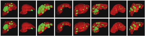
Tab. 4 gives the Dice per case for liver and tumor segmentation obtained by the proposed LW-HCN model and other state-of-the-art methods on the 3D-IRCADb dataset. It reveals that LW-HCN achieves the most accurate tumors segmentation and second-most accurate segmentation of the liver. Fig. 4 visualizes the segmentation results obtained by LW-HCN on 8 randomly selected slices and the corresponding ground truth. It shows that the results we achieved are fairly close to the ground truth. Since LW-HCN is trained on the LiTS dataset without a fine-tune on the 3D-IRCADb dataset, the impressive results shown in Tab. 4 and Fig. 4
Ground
truth
Ours demonstrate the strong generalization ability of our model.
| Methods | Tumor Dice per case (%) | Liver Dice per case (%) |
|---|---|---|
| [Foruzan and Chen, 2016] | 82.0 | - |
| [Wu et al., 2017] ∗ | 83.0 | - |
| [Moghbel et al., 2016] † | 75.0 | 91.1 |
| [Li et al., 2018a] † | 93.7 | 98.2 |
| LW-HCN (Ours) † | 94.1 | 98.1 |


5 Conclusion
In this paper, we propose the LW-HCN model to address the challenge of high computational complexity and low segmentation accuracy of 3D networks for the liver tumor segmentation. We use 2D convolutions at the bottom of the network to reduce the complexity and use 3D convolutions in the rest to capture the high-level semantic information in both spatial and temporal dimensions. To further reduce the complexity, we propose the DSTS factorization for 3D convolutions, which performs convolutions over each channel while separating the spatial and temporal convolutions in parallel. Our results on the LiTS and 3D-IRCADb datasets show that the LW-HCN model achieves the state-of-the-art performance with only 3.6 million parameters and 15.3 MB in size.
Acknowledgments
This work was supported in part by the National Natural Science Foundation of China under Grants 61771397, and in part by the Science and Technology Innovation Committee of Shenzhen Municipality, China, under Grants JCYJ20180306171334997. Jianpeng Zhang, Yutong Xie, and Pingping Zhang's contributions were made when visiting The University of Adelaide.
@inproceedings{ijcai2019p593,
  title     = {Light-Weight Hybrid Convolutional Network for Liver Tumor Segmentation},
  author    = {Zhang, Jianpeng and Xie, Yutong and Zhang, Pingping and Chen, Hao and Xia, Yong and Shen, Chunhua},
  booktitle = {Proceedings of the Twenty-Eighth International Joint Conference on
               Artificial Intelligence, {IJCAI-19}},
  publisher = {International Joint Conferences on Artificial Intelligence Organization},
  editor    = {Sarit Kraus},
  pages     = {4271--4277},
  year      = {2019},
  month     = {8},
  note      = {Main track},
  doi       = {10.24963/ijcai.2019/593},
  url       = {https://doi.org/10.24963/ijcai.2019/593},
}
TY - CPAPER TI - Light-Weight Hybrid Convolutional Network for Liver Tumor Segmentation AU - Zhang, Jianpeng AU - Xie, Yutong AU - Zhang, Pingping AU - Chen, Hao AU - Xia, Yong AU - Shen, Chunhua T2 - Proceedings of the Twenty-Eighth International Joint Conference on Artificial Intelligence, IJCAI-19 PB - International Joint Conferences on Artificial Intelligence Organization PY - 2019 SP - 4271 EP - 4277 DO - 10.24963/ijcai.2019/593 UR - https://doi.org/10.24963/ijcai.2019/593 ER -Copied
Machine-readable versions of this paper, for tools and AI agents:





