Efficient Algorithms for Learning Revenue-Maximizing Two-Part Tariffs

1 Introduction

A two-part tariff (TPT) consists of an up-front lump sum fee p1 and a fee p2 for every additional unit purchased. Various goods and services are priced using such a scheme. For example, Keurig sells coffee machines (the up-front fee) that require proprietary coffee pods (the per unit fee). Another example is health club memberships, where participants often are required to pay an up-front fixed membership fee, as well as a monthly fee. More generally, a length L menu of TPTs is a list ((p11 , p12 ), . . . , (pL1 , pL2 )) of L TPTs, and a buyer may elect to pay according to any one of the L TPTs (or not to buy anything). Menus of TPTs are also prevalent: health clubs, amusement parks, wholesale stores like Costco, cell phone companies, and credit card companies all frequently offer various tiers of membership usually consisting of lower future payments for a larger up-front payment.

In an early analysis of TPTs, Oi [1971] inspires the problem via Disneyland trying to decide between charging attendees a hefty entrance fee and allowing them free access to rides, versus charging a nominal entrance fee but requiring payment for each ride. An even earlier discussion of TPTs is given by Lewis [1941], where the merits and drawbacks of TPTs are discussed in contexts such as the telephone system, gas legislation, and the UK Central Electricity Board.

We study the problem of learning high-revenue menus of TPTs from buyer valuation data. This can be viewed as a form of automated mechanism design [Conitzer and Sandholm, 2002]. In our setting, the seller has access to samples from the distribution over buyers' values, but not an explicit description thereof. This differs from the usual approach taken by the economic theory literature, and instead takes the sample-based approach to mechanism design, introduced by Sandholm and Likhodedov [2004; 2005; 2015]. Balcan, Sandholm, and Vitercik [2018] study the sample complexity of revenue maximization, deriving a broad characterization of the number of samples needed to ensure with high probability that a mechanism that achieves high empirical revenue on the samples also generalizes well, that is, achieves high expected revenue over a freshly drawn sample. Our main goal is to provide efficient algorithms for finding menus of TPTs that achieve high empirical revenue over a given set of samples. Many of the mechanism settings studied by Balcan et al. have large parameter spaces and require a number of samples that is exponential in the problem parameters to guarantee generalization. However, they show that the sample complexity of TPTs has only a mild (at most linear) dependence on the parameters, so it is reasonable to ask for sample efficient and computationally efficient algorithms for finding nearly optimal solutions. We present such algorithms, thereby providing the missing, complementary piece to the results of Balcan et al. Our algorithms also have the obvious practical uses in designing TPTs and menus thereof.

1.1 ProblemFormulation

In our model, the seller has K units of a good to sell among n buyers j ∈ {1, . . . , n} via a menu of TPTs. Each buyer is described by his valuation function vj : {1, . . . ,K} → R over the K units. So, vj(q) is the value that buyer j assigns to getting q units of the item. (We implicitly assume that each buyer's value for getting nothing is zero.) We assume that buyers act in a utility maximizing manner: when presented with a menu ((p11 , p12 ), . . . , (pL1 , pL2 )) of TPTs, buyer j with valuation function vj : {1, . . . ,K} →Rwill choose to buy q units priced by tariff r to maximize vj (q)-(pr1+q·pr2 ), buying 0 units if there are no values of q and r that make the above expression non-negative. Given one sample of buyers v = (v1, . . . , vn), when faced with menu p, say buyer j purchases quantity qj of tariff rj. Then the revenue of p with respect to v, denoted Revv(p), is ∑nj=1 1(qj ≥ 1) · (prj 1 + qj · prj 2 ). 1

However, the model above allows for the possibility that the total quantity ∑nj=1 qj is larger than K. To deal with this issue, we will usually stipulate that the seller offers a menu p that is feasible (that is, the total quantity purchased is at most K) for each sample he sees (and we show that doing so ensures with high probability that the menu p is also feasible on a freshly drawn potential future sample).

We also study the case where each buyer belongs to one of M markets, in which case a TPT pricing scheme is of the form (p1, . . . , pM), where buyers in market m are offered menu pm. Revenue is defined similarly, which we denote by Revv(p1, . . . , pM). For a set of samples S = {v1 , . . . , vN }, the empirical revenue of p with respect to S is denoted by ̂ RevS(p) = 1N ∑Ni=1 Revvi (p), and similarly for the marketsegmented case.

We now state the formal generalization guarantee of Balcan, Sandholm, and Vitercik [2018] for the mechanism class of length-L menus of TPTs for selling K units to n buyers partitioned into M markets. Let D be some unknown distribution over n-tuples of buyer valuations and markets. For any 0 < ε, δ < 1, there exists an NTPT (ε, δ) ∈ N such that for all N ≥ NTPT (ε, δ), it holds with probability at least 1 - δ over the draw of S = {v1 , . . . , vN } ∼ DN that for every M-tuple (p1, . . . , pM) of length L menus of TPTs,

The sample complexity NTPT (ε, δ) is at most Oε,δ(MLlog(nKL)), where we have hidden the dependence on ε and δ as is typical in learning theory. This follows from the piecewise structure of the class of revenue functions: there is a partition of the TPT parameter space R2LM by hyperplanes into not-too-numerous regions such that empirical revenue is linear over each region (this notion is formalized in the main result of Balcan et al. [2018]).

The overarching goal of our paper is to efficiently find TPT pricing schemes that maximize empirical revenue over a set of samples-which by the above uniform convergence result is highly likely to be nearly optimal in terms of expected revenue as well. The number of samples needed to guarantee generalization only depends at most linearly in the problem parameters, so computationally efficient algorithms for empirical revenue maximization in this setting will be sample efficient as well.

1 We use boldface p ∈ R2L to abbreviate a menu of L TPTs. It is understood, then, that pr1 and pr2 denote p2r-1 and p2r, respectively.

1.2 Summary of the Contributions of this Paper

In Section 2 we give efficient algorithms for finding the empirical revenue maximizing menu of TPTs when the menu length is a fixed constant. Our main result here is an O(N 3K3 ) algorithm when L = 1 in the single buyer setting, that generalizes to an O(n3N 3K3 ) algorithm in the multibuyer setting (Section 2.1). We then give an (NK)O(L) algorithm for the setting where L ≥ 1 (Section 2.2). This algorithm exploits the geometric structure of the problembuyers' valuations partition the parameter space into several convex polytopes, and revenue maximization over each polytope reduces to solving a linear program.

In Section 3 we generalize the problem to multiple markets. We prove how many samples suffice to guarantee that a two-part tariff scheme that is feasible on the samples is also feasible on a new problem instance with high probability. We then show that computing revenue-maximizing feasible prices is hard even for buyers with additive valuations. Then, for bidders with identical valuation distributions, we present a condition that is sufficient for the two-part tariff scheme from the unsegmented setting to be optimal and feasible for the market-segmented setting. Finally, we prove a generalization result that states how many samples suffice so that we can compute the unsegmented solution on the samples and still be guaranteed that we get a near-optimal solution for the market-segmented setting with high probability.

1.3 Additional Related Research

(Menus of) two-part tariffs have been studied in economics [Feldstein, 1972; Ng and Weisser, 1974; Leland and Meyer, 1976; Murphy, 1977; Maskin and Riley, 1984; Wilson, 1993; Armstrong and Vickers, 2001; Sundararajan, 2004; Shi et al., 2009]. The approach taken by much of the economic literature on this topic is rather different from the perspective we pursue: most work aims to find closed-form solutions for revenue maximizing two-part tariff menus, and in attempting to do so often places various (strong) restrictions on the setting. For example, Kolay and Shaffer [2003] derive closed forms for the profit-maximizing length-two menu of two-part tariffs when there are exactly two types of buyers. Bagh and Bhargava [2013] derive further closedform results when valuations come from a finite discrete distribution. They moreover consider three-part tariffs-which has an additional quantity allowance after which the per-unit price takes effect. Schlereth et al. [2010] study some algorithmic aspects of finding revenue-maximizing TPTs. They cast the revenue-maximization problem as a mixed integer linear program and compare the performance of a few different heuristic solution algorithms. We can also write a mixed integer linear program to solve revenue maximization in our setting, but the algorithms we pose are more efficient. Other works consider two-part tariff pricing in relation to, for example, uncertainty [Lambrecht et al., 2007; Png and Wang, 2010], opportunism [Marx and Shaffer, 2004], and other practical buyer behavior [Narayanan et al., 2007; Iyengar et al., 2008]. To our knowledge, all prior work in economics considers continuous models, where quantity purchased is a continuous parameter and valuations are continuous and differentiable functions of quantity. Our setting considers a discrete and finite model, which is what gives rise to the interesting algorithmic challenges we tackle. In addition, the various examples of TPT pricing in the real world previously mentioned involve discrete quantities of goods, so our model is arguably a more realistic description of TPT pricing. TPTs have received some recent attention in computer science as well. Chawla and Miller [2016] study a form of TPTs (that is different from ours) in the context of finding simple mechanisms that yield (multiplicative) approximations to optimal revenue. However, they assume that the seller knows the distribution over buyers' values, and the mechanism design is tuned to that distribution. Notions of menu complexity and market segmentation have also been studied by computer scientists, though in different contexts [Babaioff et al., 2017; Hart and Nisan, 2019; Cummings et al., 2020].

To our knowledge, the only prior work that studied the model of TPTs that we address is that of Balcan et al. [2018]. However, they only studied sample complexity rather than algorithms. We take this a step further and solve the learning problem efficiently in terms of computation.

2 Algorithms for Optimal TPT Structures

In this section we study the computation of TPT structures that maximize empirical revenue over the given set of samples. We are given a set of samples S = {v1 , . . . , vN }, where each sample vi = (vi1 (1), . . . , vi1 (K)), . . . , (vin (1), . . . , vin (K)). That is, each sample gives a value for each buyer for each number of units bought. In the sample-based mechanism design literature, it is standard to assume a complete valuation draw like this in each sample. We also use the shorthand vij = (vij (1), . . . , vij (K)). In the first subsection we discuss computation of a single TPT and in the next subsection computation of a menu of multiple TPTs. In both sections we discuss the single-buyer case for simplicity, and then in the third subsection we present the generalization to the multi-buyer case.

2.1 An Efficient Algorithm for a Single TPT

In this subsection we give a polynomial-time algorithm to solve the empirical revenue maximization problem in the case where we can offer only one two-part tariff, that is, the menu length L = 1. Because in this section we are presenting the single-buyer case for simplicity, we do not include the buyer subscript in the valuations. So, our input is S = {v1 , . . . , vN } = {(v1 (1), . . . , v1 (K)), . . . , (vN (1), . . . , vN (K))}.

We observe the following, which is key for our algorithm.

Lemma 1. Suppose (p1, p2) is a TPT that maximizes empirical revenue over S. Then, the line with y-intercept p1 and slope p2 passes through a point (q, vi (q)) for some i ∈ {1, . . . , N} and q ∈ {1, . . . ,K}.

Proof. Consider a TPT line with y-intercept p1 and slope p2 that does not pass through any such point. Let d > 0

be minimal such that the TPT line with y-intercept p1 + d and slope p2 passes through such a point. For any buyer j, argmaxq vj (q) - (p1 + p2q) = argmaxq vj (q) - (p1 + d + p2q), so any buyer who was purchasing a nonzero quantity q when faced with (p1, p2) continues to purchase quantity q when faced with (p1+d, p2). Any buyer who purchased nothing when faced with (p1, p2) clearly continues to purchase nothing. Hence the TPT (p1 + d, p2) generates strictly more revenue than (p1, p2).

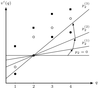
Now, for each point (q, vi (q)), we demonstrate that to find the revenue-maximizing tariff line it suffices to search over a set of at most NK tariff lines passing through (q, vi (q)). Suppose we have a tariff line passing through (q0, vi0 (q0)), at which buyer i buys quantity qi. Let us compute the slope p2 of such a tariff line at which i prefers to buy quantity q over qi. We have

For i, q, q′ let αi0,q0 (i, q, q′ ) = vi (q)-vi (q′ ) q-q′ denote the slope where buyer i switches preferences between quantity q and q′ (this has no dependence on i0 and q0, but for notational consistency we leave the subscript). We must also account for the case where buyer i switches preferences between quantity q and purchasing nothing, for which a similar calculation gives αi0,q0 (i, q, 0) = vi (q)-vi0 (q0) q-q0 .

The algorithm works by "hinging" a TPT at every point of the form (q, vi (q)), and then increases the slope of the tariff line at increments determined by the α values-these increments represent thresholds at which some buyer starts buying a different quantity. As the slope of the hinged tariff line increases, the quantity purchased by a given buyer changes at most K times, and hence there are at most NK slope thresholds to check-between any two thresholds the average revenue is linear in the TPT since the quantities purchased are constant, and so the maximum revenue must be attained at one of these thresholds. See Figure 1 for an illustration. We write down the precise algorithm as Algorithm 1.

Theorem 1. Algorithm 1 finds the single tariff (p1, p2) that maximizes empirical revenue over a sample set of size N in O(N 3K3 ) time.

Proof. That the algorithm finds the maximum revenue TPT follows from the fact that if p2 < p′2 are two consecutive slopes checked by the algorithm, the average revenue is linear as the slope varies between p2 and p′2 (revenue is linear since, by construction, the quantities purchased by each buyer are constant for slopes varying between p2 and p′2 ) and hence it suffices to compute revenue at the endpoints. Lemma 1 shows that the empirical revenue maximizer passes through a point (q, vi (q)), and since Algorithm 1 checks all slope thresholds for TPTs passing through each such point, we are guaranteed to find the TPT yielding the maximum empirical revenue.

We now count the number of steps taken by Algorithm 1. Line 2 involves NK iterations, Line 4 involves N iterations, Line 9 involves at most NK iterations (since each buyer starts by purchasing K units, and can change quantities at most K times as the slope p2 increases), computing the minimization in Lines 10 and 11 requires at most NK steps, and computing revenue in Line 14 requires N steps. So the total run time is O(NK(N + NK(NK + N))) = O(N 3K3 ).

We ran Gurobi (the fastest general-purpose mixed integer program solver) to find the revenue-maximizing single TPT for a single buyer (after formulating this problem as an integer program), and Algorithm 1 beat it dramatically. For example, averaged over 10 runs on randomly generated instances with K = 5 units and N = 600 samples, our algorithm returned the revenue-maximizing TPT in under 23 minutes while Gurobi took over 3.5 hours.

2.2 An Algorithm for Multiple TPTs

In this subsection we give an algorithm for optimizing a menu of two-part tariffs. Inmost applications, for practical reasons, the length of the menu cannot be very long, so L is a small constant (typically 2 or 3). We present an algorithm that is exponential in L but still polynomial in N and K. It can be viewed as a generalization of the single tariff algorithm. The geometric structure of the problem is the same as in Balcan et al. [2018], but we exploit it to get algorithms while they use it to prove sample complexity bounds.

Theorem 2. There is an algorithm that finds the empirical revenue maximizing length L menu of tariffs over a sample set of size N in (NK)O(L) time.

Proof. For input valuations v1 , . . . , vN , let Hi(q, q′ , r, r′ ) denote the hyperplane

where if q (or q′ ) is 0, the LHS (or RHS) is replaced by 0. Consider the collection of hyperplanes H consisting of these (at most N(KL)2 ) hyperplanes for each q, q′ ∈ {0, . . . ,K}, r, r′ ∈ {1, . . . ,L}, i ∈ {1, . . . ,N}. It is a basic combinatorial fact that H partitions R2L into at most |H|2L ≤

Algorithm 1 Single TPT for a Single Buyer

Input: Set of samples S = {v1 , . . . , vN }

Output: TPT (p1, p2) maximizing empirical revenue over S

• 1: Initialize MaxRev ← 0.
• 2: for (i, q) ∈ {1, . . . ,N}×{1, . . . ,K} do
• 3: p2 ← 0
• 4: for j ∈ {1, . . . ,N} do
• 5: if vj (K) ≥ vi (q) then

qj ← K (This makes the typical assumption that each buyer's valuation is nondecreasing in quantity. If that is not the case, one can in this line simply loop over quantities for each buyer separately in order to find the utility-maximizing quantity

• 6: for that buyer.)
• 7: else
• 8: qj ← 0
• 9: repeat

• 12: qj ∗ ← q∗

• 14: MaxRev ←max{MaxRev, ̂ RevS(p1, p2)}
• 15: until no update is found
• 16: return revenue maximizing (p1, p2)

N 2LK4L regions (each region is a connected component of R2L \ ∪i,q,q′ ,r,r′Hi(q, q′ , r, r′ ) and is an intersection of at most |H| halfspaces). The average revenue over the set of samples is linear within each such region, since the quantity purchased by each buyer remains constant within each region, so the maximum revenue within a region C can be found by solving the following linear program: if buyer i purchases quantity qi(C) ∈ {0, . . . ,K} of tariff ri(C) ∈ {1, . . . ,L} within C, the maximum revenue in C is

Each linear program involves 2L real variables, and |H| ≤ NK2 constraints. So, it can be solved in poly(N,K, L) time.

Moreover, there is a simple algorithm with run time poly(N 2LK4L) which outputs a representation of each region determined by H as a 0/1 vector of length |H|, where the kth entry determines on which side of the kth hyperplane of H the region lies on. The high-level idea is to sequentially add each hyperplane to the list of regions maintained so far (starting with the entire Euclidean space R2L), iterating over the current regions and checking whether the added hyperplane intersects each region-updating the list of regions if so. See [Xu, 2020] for a more detailed description of enumerating the regions formed by a collection of hyperplanes (in a totally different context). Our algorithm solves the aforementioned linear program for every such region and picks the solution that yields highest empirical revenue.

In the single TPT (L = 1) case, Algorithm 1 is more efficient than the algorithm presented in Theorem 2. This is because the former is a direct combinatorial algorithm that does not require solving LPs.

2.3 Generalization toMultiple Buyers

While our algorithms in the two subsections above were presented in the single buyer setting, they directly extend to the multi-buyer setting as follows.

Algorithm 1 generalizes by feeding in not just N valuations but all nN valuations. The only change to the algorithm itself is that in Step 12 we check that the allocation is feasible, that is, not more than the total quantity K is bought among the buyers in any sample i ∈ {1, . . . ,N}; if more is bought, then the assignment on that line is skipped because that pricing solution is infeasible. (Another nuance is that the initialization in Lines 2-8 might not be feasible, but that is fine.)

Similarly, in our multi-TPT algorithm, whenever we are about to solve an LP corresponding to some region determined by the set of hyperplanes, we first check that the region is feasible in the sense that the total quantity bought by buyers in any one sample is at most K.

Remark. Suppose buyers have additive valuations, that is, vi (q1+q2) = vi (q1)+vi (q2) for any quantities q1+q2 ≤ K. Then, the revenue maximization problems considered in this section become trivial. In particular, the run time dependence on K and L vanishes. This can be seen due to the fact that price(q) := minr pr1 +q · pr2 is a piece-wise linear increasing concave function. An additive buyer's valuation function is simply a line with positive slope passing through the origin, as vi (q) = vi (1 + · · · + 1) = q · vi (1). Hence, the difference vi (q) - price(q) is always maximized when q = K, that is, buyers are always only interested in the entire K-unit bundle. Thus, revenue is determined by a single price, that of the entire bundle, and the seller simply can try every possible price in {v1 (K), . . . , vN (K)}, due to Lemma 1.

3 Market Segmentation

We now consider a setting in which each buyer belongs to one of M markets X1, . . . ,XM-determined by attributes such as geographic location, income level, etc. The seller sets M length L-menus of TPTs (p1, . . . , pM), where buyers in market m are allowed to purchase according to pm.

The seller wants to offer a TPT menu for each market so that the overall solution across markets is feasible, that is, that the sum of the demands of the markets does not exceed K. We show that any solution that is feasible for each sample in a large enough sample set is with high probability a feasible solution for any future sample.

Proposition 1. Let N ≥ NTPT (ε, δ). With probability at least 1-δ over the draw of S ∼ DN , if p1, . . . , pM is feasible for S,

Proof. Consider the class of 0/1 valued indicator functions {fv(p1, . . . , pM)} indicating whether (p1, . . . , pM) is feasible for v. For a single sample i, consider the set of hyperplanes of the form

for each j, q, q′ , r, r′ , where m(i, j) is the market to which buyer j in sample i belongs. These hyperplanes partition the tariff space R2LM into at most (n(KL)2 )2LM regions such that the indicator is constant within each region. Thus, by Theorems 2.2 and C.1 of Balcan et al. [2018], for a sample set S of size at least NTPT (ε, δ), it holds with probability at least 1 - δ that for all p1, . . . , pM,

So, if (pS1 , . . . , pSM ) is any feasible solution for S, that is, ̂ fS(pS1 , . . . , pSM ) = 1, we have

with probability at least 1 - δ over the draw of S and v.

It turns out that market segmentation introduces substantial computational hurdles to revenue maximization. Even when bidders are additive (which removes the parameters L and K from the problem as remarked in the previous section), the problem of setting a feasible price for each market in an empirical revenue maximizing way is NP hard. Since additive buyers either purchase the entire bundle of K units or nothing, each menu is reduced to a single price, so the seller's problem is to set prices p1, . . . , pM for each market. Any solution must be feasible for the set of samples, which means at most one buyer can purchase the full K units in each sample.

Theorem 3. Consider a set of samples S = {v1 , . . . , vN } where each buyer belongs to one of M markets. Even if all buyers have additive valuations, there is no algorithm that finds feasible prices p1, . . . , pM that maximize empirical revenue over S in time polynomial in M and N, unless P = NP.

Proof. We reduce from Maximum Weight Independent Set. Given an instance G = (V,E) of Maximum Weight Independent Set (without loss of generality assume G has no isolated vertices), label the vertices V = {v1, . . . , vn}, and let wi = weight(vi). Let pi = wi|E| deg(vi) . We will have n markets X1, . . . , Xn, corresponding to the vertices of G.

For each (vi, vj) ∈ E, we introduce a sample consisting of a buyer in market Xi with value pi and a buyer in market Xj with value pj (ensuring that no feasible pricing solution can simultaneously offer pi to market Xi and pj to market Xj). So we have a total of |E| samples. Clearly, any feasible revenue maximizing solution involves offering market Xi either price pi, or something higher than pi (so that no buyer in market Xi across any of the samples makes a purchase).

Our construction yields a one-to-one correspondence between independent sets in G and feasible n-tuples of prices: an independent set I ⊆ V with weight W = ∑vi∈I wi corresponds to a pricing solution where if vi ∈ I, market Xi is offered pi, and if vi /∈ I, market Xi is offered something higher than pi. For a vertex vi in the independent set, there are precisely deg(vi) samples containing a buyer in market Xi who makes a purchase at price pi, so the average revenue obtained by the pricing solution corresponding to I is 1 |E| ∑vi∈I deg(vi) · pi = W, by the choice of pi. This completes the (clearly polynomial time) reduction.

Remark. This hardness is inherent to the limited supply setting. If the seller has unlimited supply, and K is instead the maximum quantity any buyer is willing to purchase, we can find the empirical revenue maximizing market-segmented solution in M(nNK)O(L) time simply by running the procedure described in the previous section restricted to each market in turn. This finds the empirical optimum over each market, and without capacity constraints, this is a feasible solution and thus the optimal market-segmented solution as well.

3.1 Buyers with Identically Distributed Valuations

To circumvent the hardness of feasible empirical revenue maximization over worst case instances, we now study a setting where each buyer's valuation vector is drawn from the same distribution. Each market is of a certain prescribed size, and buyers are indistinguishable across markets. An example of a natural real-world market segmentation that potentially satisfies this is segmentation based on geographic location. For example, there may be no reason to believe that the average buyer in San Francisco values a gym-membership plan any differently than the average buyer in Pittsburgh. We show that under certain conditions, it is optimal to treat every buyer equally-regardless of whether they come from a large market or a small market. This immediately yields a simple algorithm in which we solve the non-segmented version of the problem, and reuse the solution for the segmented version.

Suppose there are a total of n buyers across markets, and an αm fraction of these buyers belong to market Xm. For simplicity, we assume that the seller receives zero revenue on instances on which the chosen solution is infeasible. Suppose the optimal solution (p∗1 , . . . , p∗M ) = argmax(p1,...,pM) Ev[Revv(p1, . . . , pM)] satisfies the property that in expectation, buyers from market Xm contribute an αm fraction of the total revenue. That is, Ev[Revv|Xm (p∗m)] = αm · Ev[Revv(p∗1 , . . . , p∗M )] for each m. In this case, we can reuse the non-segmented solution. For a randomly drawn v, let F denote the event that fv(p∗1 , . . . , p∗M ) = 1. We have that

so Ev[Revvm (p∗m) | F] = 1n Ev[Revv(p∗1 , . . . , p∗M ) | F] for each m. Thus, we can set p∗1 = · · · = p∗m, and hence we only need to search for an optimal solution in the non-segmented case that we then offer to every market. The empirical revenue maximizing menu of TPTs p in the non-segmented case can be computed in (nNK)O(L) time, as in the previous section. Finally, we provide the generalization guarantee for using the unsegmented solution in the market-segmented case.

Theorem 4. Let N ≥ NTPT (ε, δ). In the above setting, with probability at least 1 - δ over the draw of S ∼ DN ,

where p is the empirical revenue maximizing solution when all the markets are combined.

Proof. Let p∗ denote the expected revenue maximizer in the non-segmented case, so by the previous discussion, (p∗ , . . . , p∗ ) is also the expected revenue maximizer in the segmented case. Theorem C.1 of Balcan et al [2018] yields |̂ RevS(p) -Ev[Revv(p)]|, |̂ RevS (p∗ ) - Ev [Revv (p∗ )| ≤ ε with probability at least 1 - δ over the draw of S. As ̂ RevS(p) ≥ ̂ RevS(p∗ ) and Ev[Revv(p∗ )] ≥ Ev[Revv(p)], applying the triangle inequality yields the result.

4 Conclusions and Future Research

TPTs are a frequently-used pricing scheme in many applications. In this paper we studied efficient algorithms for finding revenue-maximizing TPT pricing schemes in the setting where the buyers' valuation distributions are given via samples. These algorithms have clear direct uses. They also provide the missing piece in the recent generalization theory for TPTs [Balcan et al., 2018], which also uses samples of valuations as the input, and whose generalization approach is based on revenue-maximizing TPT schemes, but which did not provide any algorithms for computing such schemes.

We presented a polynomial algorithm for the case of optimizing one TPT. We also presented an algorithm for optimizing length-L menus of TPTs with complexity exponential only in L and polynomial in the other problem parameters.

We then generalized the problem of designing TPT schemes to multiple markets. We first proved how many samples suffice to guarantee that a TPT scheme that is feasible on the samples is also feasible on a new problem instance with high probability. We then showed that computing revenuemaximizing feasible prices is hard even for buyers with additive valuations. Then, for bidders with identical valuation distributions, we presented a sufficient condition for the TPT scheme from the unsegmented setting to be optimal and feasible for the market-segmented setting. Finally, we proved a generalization result that states how many samples suffice so that we can compute the unsegmented solution on the samples and still be guaranteed that we get a near-optimal solution for the market-segmented setting with high probability.

Several interesting open questions arise from our work. Can the (NK)O(L) algorithm in Theorem 2 be improved? In particular, can the exponential dependence on L be improved, or is the problem NP-hard? Moreover, the algorithm given in that theorem is fairly general purpose, and is not restricted to menus of TPTs. Can our method be used to develop efficient algorithms for other mechanism design settings? In the realm of market segmentation, are there interesting structural connections between the distributions over buyers' valuations in each market and potential polynomial time algorithms?

Acknowledgements

This material is based on work supported by the NSF under grants IIS-1718457, IIS-1617590, IIS-1901403, CCF1733556, CCF-1535967, CCF-1910321, and SES-1919453, the ARO under award W911NF-17-1-0082, the Defense Advanced Research Projects Agency under cooperative agreement HR0011202000, an AWS Machine Learning Research Award, an Amazon Research Award, a Bloomberg Research Grant, and a Microsoft Research Faculty Fellowship.