Convexified Graph Neural Networks for Distributed Control in Robotic Swarms

1 Introduction

Nowadays, data networks are everywhere to be found due to the arising networking revolution. Networks model entities in a wide variety of domains, such as communication networks, biology, and sociology. Unique to swarm robotics, data exhibits irregular and complex structures, provoking existing linear methods. Modeling data networks as graphs, whereas the data is viewed as a signal on top of it, Graph Signal Processing (GSP) [Ortega et al., 2018] expands the concept of graph convolutions, which account for the underlying graph structure during the processing of data. Built upon the GSP's goal, Graph Neural Networks (GNNs) constitute nonlinear representation maps with capability of exploiting those underlying structures [Gama et al., 2020]. As in most neural networks, GNNs are then trained by solving a nonconvex Empirical Risk Minimization (ERM) problem, which is known to be NP-hard [Blum and Rivest, 1992].

Considering the problem of controlling a robotic swarm in dynamic settings with different initial positions and velocities, as well as topology changes, yields a difference in structures between training and testing due to the dynamic nature of the system. GNNs have been proven to have the fundamental properties of permutation equivariance and stability to changes in the topology [Gama et al., 2020].

For improving the performance, Online Learning constitutes an appropriate solution, providing us with adaptive optimization algorithms suitable for continuously time-varying topologies [Dabbagh and Bannan-Ritland, 2005]. Yet, it requires the convexity of both the domain and the loss function. However, ERM on a nonlinear neural network model is generally non-convex, as on GNNs. Thus, this paper introduces convexified GNN architectures, which are well-suited for both online algorithms and real-world applications, in which data can be naturally represented as graphs (e.g., recommendation systems [Gao et al., 2020]), while maintaining convergence guarantees. Following [Zhang et al., 2017], we first illustrate a convex relaxation when regarding linear activation functions. For the nonlinear case, we then propose a relaxation to a suitably chosen Reproducing Kernel Hilbert Space (RKHS), reducing the problem to the linear case. Finally, we demonstrate in rigorous experiments the superiority of the convexified GNN solutions over existing solutions for formation control in a swarm of robots in terms of faster convergence rate, up to an expected generalization error.

2 RelatedWork

[Li et al., 2019] concern with the problem of collision-free navigation in multi-robot systems, where the robots possess limited sensing and no global reference frame for localization. They compose a Convolutional Neural Network (CNN), which extracts adequate features from local observations, and a GNN that communicates these features among the robots. [Sartoretti et al., 2019] assume no explicit communication. Yet, both researches are restricted to zero communication time-delay. Accordingly, [Tolstaya et al., 2020] offer the use of Aggregation GNNs [Gama et al., 2018a] (A-GNNs) to operate on time-varying graph processes. Both papers utilize Imitation Learning, and rely on the availability of an optimal solution (i.e., expert data). Furthermore, they each run one GNN per time instant, posing a high computational expense, which thus requires shallow GNNs and short filters.

Online learning is vastly explored in the context of neural networks [Li et al., 2004; Hong et al., 2015]. [Gao et al., 2020] tackle the convexity requirement of online algorithms by proposing the Wide and Deep GNN (WD-GNN), consisting of two components: a wide component (which is a bank of graph filters), and a deep component (which is a GNN). They solely retrain the linear wide component, whereas the deep one remains fixed after the training phase. Yet, their solution is limited to the extent of linear transforms and does not involve online retraining of the GNN. As opposed to their work, we retrain the GNN part as well.

[Nikolentzos et al., 2018]'s approach to the graph classification problem is similar to our own: they extract patches from each input graph via community detection, embed them with graph kernels and then feed them through a 1D CNN, to which pooling is applied. A fully-connected layer with a softmax completes the architecture. Community detection algorithms, which partition a network into clusters of densely connected nodes, are known to be computationally intractable and require a large storage space [Blondel et al., 2008]. We thus leverage the graph signal processing (GSP) concepts for learning from graph signals (via GNNs) [Ortega et al., 2018], rather than communities. Additionally, as opposed to their one-layered model, ours are multi-layered.

Notations. For brevity, [n] denotes the discrete set {1, 2, . . . , n} for any n ∈ N>0. For a rectangular matrix A, let ||A||∗ be its nuclear norm, and ||A||2 be its spectral norm (i.e., maximal singular value). Let L2 (N) denote the set of countable dimensional vectors v such that ∑∞i=1 vi < ∞.

3 GNNs - Background

Let G = (V, E,W) be the underlying graph structure, where: V = {1, ..., n} denotes the vertex set, E denotes the edge set and W : E → R denotes the edge weight function, where a missing edge (i, j) is depicted by W(i, j) = 0. The neighborhood of node i ∈ V is denoted by Ni := {j ∈ V|(j, i) ∈ E}. Following [Ortega et al., 2018], we leverage the graph signal processing (GSP) concepts for deriving the foundation of learning from graph signals. Thus, the data X ∈ Rn×F is modeled as a graph signal where [X]i = xi constitutes an F-dimensional feature vector, assigning a state for node i ∈ V. In the context of swarm robotics, this state is typically described by the agent's position, velocity or acceleration. For the sake of relating the the graph signal X with the underlying structure of G, we define a graph shift operator (GSO) by S ∈ Rn×n , which correlates to the graph's sparsity and satisfies [S]ij = sij = 0 if (j, i) /∈ E for j ̸= i. Commonly utilized GSOs include the adjacency matrix [Sandryhaila and Moura, 2013; Sandryhaila and Moura, 2014], which corresponds to either directed or undirected graphs, the Laplacian matrix [Shuman et al., 2013], which solely applies to undirected graphs, and their normalized counterparts [Defferrard et al., 2016; Gama et al., 2018b]. Hence, we clarify that the consideration of either a directed or an undirected graph is with close proximity to the choice of the GSO. The graph signal X can be shifted over the nodes by viewing S as a linear operator, yielding that the output at node i for the f th feature becomes:

The second equality thereby emphasizes the sparsity nature (or, more accurately, locality) of S. We shall observe that, whereas SX corresponds to the local information exchange between a given node and its direct neighbors, applying this linear operator recursively yields information from nodes in further hops along the graph, i.e., the k-shifted signal S kX constitutes the aggregation of information from nodes which are k-hops away. Hence, given a set of filter taps H := {Hk ∈ RF×G}Kk=0 , a graph (convolutional) filter [Ortega et al., 2018] with G output features can be defined as a linear combination of data located at consecutive hops:

where the output is another graph signal of order n×G, over the same graph. Feeding a graph filter into a pointwise nonlinear activation function yields a Graph Neural Network (GNN) [Gama et al., 2020]. It is defined as a nonlinear mapping between graph signals Φ : Rn×F → Rn×G given by:

where ℓ ∈ [L]. σ : R → R is a pointwise non-linear activation function (which, for brevity, denotes its entrywise application in (3)), and H := {Hℓk = (hfg ℓk ) ∈ RFℓ-1×Fℓ |k ∈ [K] ∪ {0}, ℓ ∈ [L]} is a set of filter taps. The graph signal Xℓ ∈ Rn×Fℓ is referred to as a graph perceptron [Gama et al., 2020], occupying the ℓth layer of a multi-layer graph perceptron generated by the cascade of all L graph signals above. The input is X0 = X, yielding F0 = F, where the output has FL = G features. Each input feature xgℓ-1 (g ∈ [Fℓ-1]) at layer ℓ is processed in parallel by Fℓ graph filters to output the following features. Given some positive constants Rℓ, which can be viewed as communication power constraints, the non-convex function class of GNNs is provided by:

3.1 Empirical RiskMinimization (ERM)

We train the GNN (3) by solving the following empirical risk minimization (ERM) problem for some loss function J : Rn×G →R and a training set T := {X (j) }mj=1 :

The number of parameters H to be trained is determined by the number of: layers L, filter taps K and features Fℓ in the ℓth layer. Abusing the notation slightly, we regard (5) as capable of coping with supervised problems, due to the possible extension of J to operate on the optimal action as well.

4 GNNs Convexification

Since Fgnn (4) forms a non-convex set and due to the nonlinearity of the activation function, the ERM problem on GNNs is non-convex, yielding that: (1) their training process is NP-hard, and (2) they are unsuitable for online learning. Hence, we aim at overcoming this issue by convexifying both the ERM's predictions domain and loss function. Following the method put forth by [Zhang et al., 2017] for Convolutional Neural Networks (CNNs), we develop the class of Convexified GNNs (Cx-GNNs). As a first step, in Section 4.1 we illustrate a convex relaxation of a low-rank constraint based on the nuclear norm when regarding linear activation functions. In the nonlinear case (Section 4.2), we propose relaxation to a suitably chosen Reproducing Kernel Hilbert Space (RKHS), where the resulting relaxed filters satisfy a low-rank constraint, reducing the problem to the linear case.

4.1 Linear Activation Functions

In this section, we employ the nuclear norm in the simple case of the linear activation function σ(w) = w (yielding xfℓ = ufℓ due to (3)), which provides us with a convex function class, as opposed to (4). Indeed, consider the eigenvector decomposition of the shift operator S = VΛV T , with orthogonal eigenvectors matrix V := [vi]ni=1 and distinct eigenvalues matrix Λ := diag[λi]ni=1 , in ascending order. For each filter (1 ≤ f ≤ Fℓ, 1 ≤ g ≤ Fℓ-1):

where Hfg ℓ (Λ) = diag[hfg ℓ (λi)] for hfg ℓ : R → R given by hf g ℓ (λ) = ∑Kk=0 hfg ℓk λk , which satisfies (from (4)):

Note that {hfg ℓ (λi)vi}ni=1 would be less than n if and only if λi is a root of the polynomial hfg ℓ (λ), i.e., rk(Hfg ℓ (Λ)) ≤ n. From (3) and (6), xfℓ can be written as follows:

where, in the last step, we have defined the Fℓ-1×Fℓ-1 block matrix ˜Hf ℓ := diag[VHfg ℓ (Λ)V T ]Fℓ-1 g=0 . Hence, xfℓ linearly depends on ˜Hf ℓ , whose rank satisfies (rk(Hfg ℓ (Λ)) ≤ n):

Let ˜Hℓ := [ ˜Hf ℓ ]Fℓ f=1 . From (9), we clearly infer:

whereas Xℓ can be written as:

As in [Zhang et al., 2017], the nuclear norm of ˜Hℓ is a convex relaxation of its rank constraint. In the supplementary material, we provide a rigorous proof, yielding:

Hence, defining the function class for Cx-GNN:

it is guaranteed that Fgnn ⊆ Fcx-gnn. Consequently, solving the ERM (5) over Fcx-gnn instead of Fgnn yields a convex optimization problem over a wealthier class of functions.

4.2 Nonlinear Activation Functions

Following [Zhang et al., 2017], for certain nonlinear activation functions σ and suitably chosen kernel functions K, we prove that the class of GNNs can be relaxed to a Reproducing Kernel Hilbert Space (RKHS), reducing the problem to the linear activation case. Full proofs are omitted due to space constraints, and can be found in the supplementary material (https://u.cs.biu.ac.il/∼agmon/IJCAI21Sup.pdf). Furthermore, readers should refer to [Sch¨olkopf et al., 2001] for a brief overview on RKHS.

Let hfg ℓ : R→R be given by hfg ℓ (λ) = ∑Kk=0 hfg ℓk λk . Let K : Rn ×Rn → R be a positive semidefinite kernel function. We are able to show that (wf ℓ (i) := ∑Fℓ-1 g=0 hfg ℓ (λi)ei):

Hence, regarding certain choices of kernels and a sufficiently smooth σ, the function τ f ℓ : z ↦→ σ((〈z,wf ℓ (i)〉)ni=1 ) is contained within the RKHS induced by the kernel function K. From the representer theorem, provided a sufficiently smooth σ, and in regard with a certain choice of kernel K, there exists a feature mapping ϕ : Rn → L2 (N) for which K(z, z′ ) = 〈ϕ(z), ϕ(z′ )〉. From (14) (i ∈ [n]):

where ¯wf ℓ (i) ∈ L2 (N) is a countable-dimensional vector, due to the fact that ϕ itself is a countable sequence of functions. Regarding the supplementary material, we have that || ¯wf ℓ (i)||2 ≤ Cσ(||wf ℓ (i)||2), provided a monotonically increasing Cσ which depends on K. Consequently, ϕ may be utilized as the vectorized representation of the output features ufℓ , where ¯wf ℓ (i) constitutes the linear graph filter taps, thus reducing the problem to training a GNN with the identity activation function. That is, each graph perceptron is now parametrized by the countable-dimensional vector ¯wf ℓ (i).

As our next step, we shall provide a reduction of the original ERM problem to a finite-dimensional one. Output on the training data T := {X (j) }mj=1 should be solely considered when solving the ERM problem, i.e., the output of 〈ϕ(yf ℓ (j)), ¯wf ℓ (i)〉 (where yf ℓ (j) is as given in (14) for X0 = X (j) ). Without loss of generality, for the sake of solving the ERM, we assume that ¯wf ℓ (i) ∈ span{ϕ(yf ′ ℓ (j))|(j, f ′ ) ∈ [m] × [Fℓ]}. We can thus reparameterize it by:

Let αf ℓ (i) := [αf ′ ℓ,j (i)](j,f ′ )∈[m]×[Fℓ]. Hence, for estimating ¯wf ℓ (i), it suffices to estimate the vector αf ℓ (i). By definition, the relation (αf ℓ (i))T Kf ℓ αf ℓ (i) = || ¯wf ℓ (i)||22 holds, where Kf ℓ ∈ RmFℓ×mFℓ denotes the symmetric kernel matrix, whose rows and columns are indexed by the examplestate index (j, f ′ ) ∈ [m] × [Fℓ]. The entry at row (j ′ , f ′ ) and column (j ′′ , f ′′ ) equals to K(yf ′ ℓ (j ′ ), yf ′′ ℓ (j ′′ )). For a suitable approximation of Kf ℓ such that Kf ℓ ≈ QQT for Q ∈ RmFℓ×p , let Q+ be the pseudo-inverse of Q. Let vℓ(z) ∈ RmFℓ be a vector whose (j, f)th coordinate equals to K(z, yf ℓ (j)). Denoting Aℓ := [Afℓ ]Fℓ f=1 , the Cx-GNN is given as follows (in regard with (3) and (14)):

Remark 1. Note that: ˜ yf ℓ (j) = Q+vℓ(yf

ℓ (j)) = [Q]j,f .

The Cx-GNN can also be depicted by:

It can thus be proven that:

4.3 LearningMulti-Layer Cx-GNNs

Alg.1 is an abbreviated version for learning a multi-layer Cx-GNN. At each layer, given regularization parameters {Rℓ}Lℓ=1 , solving the following optimization problem is required (from (17)):

The naive approach is solving via projected gradient descent: At iteration t, for a step size ηt > 0, we compute:

where ΠRℓ denotes the Euclidean projection onto the nuclear norm ball with radius Rℓ. As in [Zhang et al., 2017], this can be done by projecting the vector of singular values onto the ℓ1-ball, and then reconstructing the matrix using the projected singular values. Afterwards, the ℓth layer output shall be retrieved: they propose to compute the singular value decomposition ˆ Aℓ = UℓΣℓW T ℓ , and then define ˜Uℓ to be the first Fℓ columns of Uℓ. The resulting output, whose (f, i)th element equals to 〈Q+vℓ(z),QT αf ℓ (i)〉, is given by:

Algorithm 1 Learning Multi-Layer Cx-GNNs

Input: Samples {X (j) }mj=1 , kernel K, {Rℓ}Lℓ=1 , number of graph filters {Fℓ}Lℓ=1 , ˜H1(z) = z

• 1: for 2 ≤ ℓ ≤ L do
• 2: Taking { ˜Hℓ-1(X (j) )}mj=1 as training examples, construct a kernel matrix Kf ℓ ∈ RmFℓ×mFℓ , such that the entry at row (j ′ , f ′ ) and column (j ′′ , f ′′ ) equals to K(yf ′ ℓ (j ′ ), yf ′′ ℓ (j ′′ )). Compute a suitable approximation of Kf ℓ such that Kf ℓ ≈ QQT for Q ∈ RmFℓ×p .
• 3: Compute ˜ Y (j) ℓ := [˜ yf ℓ (j)]Fℓ f=1 as in Remark 1 for X (j) .
• 4: Solve (21) so as to obtain a matrix ˆ Aℓ.
• 5: Compute the singular value decomposition ˆ Aℓ = UℓΣℓW T ℓ , and define ˜Uℓ as the first Fℓ columns of Uℓ.
• 6: Compute ˜ Pℓ(z) := [tr( ˆ Afℓ ˜ Yℓ(z))]Fℓ f=1 and ˜Hℓ(z) (23).

7: end for

Output: Predictor ˜ PL, output ˜HL and parameters ˆ AL.

The time complexity is affected by p. For instance, by Nystr¨om method [Williams and Seeger, 2001], an approximation of Kf ℓ is achieved by randomly sampling p ≪ mFℓ rows/columns from the original Kf ℓ in O(p2mFℓ) time.

4.4 Convergence Analysis

As in Theorem 1 of [Zhang et al., 2016], we prove the following theorem, from which we infer that the role Rℓ plays is twofold: it ensures that Fgnn ⊆ Fcx-gnn and Fcx-gnn is a wealthier class of functions, but not "too big". We denote yf ℓ (z) := ∑Fℓ-1 g=0 zg . We use the random kernel matrix K(Xℓ-1) ∈ RFℓ × RFℓ , whose (f, f ′ )th entry is given by K(yf ℓ , yf ′ ℓ ), where yf ℓ is as in (3) and the ℓth layer input Xℓ-1 ∈ Rn×Fℓ-1 is drawn randomly.

Theorem 1. Let J(·) be L-Lipchitz continuous and K be either the inverse polynomial kernel or the Gaussian kernel. For any valid activation function σ, in regard with the radius ˜ Bℓ as in (20), the expected generalization error satisfies:

at layer ℓ and for a universal constant c > 0.

Proof. (Sketch) Let ˜ Bf ℓi := Cσ((Rfg ℓ Fℓ-1sK(λi))2 ). While regarding the ℓth layer, the proof comprises of two parts: First, a wealthier function class shall be considered, which contains the class of GNNs. It is defined as follows:

where || · ||H is the associated RKHS norm. We prove that the predictor ˜ Pℓ, as computed by Alg.1, solves the ERM problem for Fcx-gnn. Afterwards, we provide an upper bound on its Rademacher complexity. After proving Fgnn ⊆ Fcx-gnn, we infer that the generalization loss of ˜ Pℓ is bounded by that of GNNs. Combined with the theory of Rademacher complexity [Bartlett and Mendelson, 2002], this loss converges to the least possible error of Fcx-gnn, establishing (24).

5 Extensions of Cx-GNNs

In this section, we extend the model proposed in Section 4 to other existing architectures found in the literature.

As a first step, we consider Aggregation GNNs (AGNNs), which apply to a signal with temporal structure, incorporating the topology of the graph [Gama et al., 2018a]. Denoting the ℓth aggregation sequence at node i by:

the ℓth layer output can be thus expressed as:

As in Section 4, leveraging the concept of convexified CNNs [Zhang et al., 2017], the class of Convexified A-GNNs (CA-GNNs) can be readily formed. Indeed, for a linear activation function, regarding (27), we infer that Z (ℓ) i linearly depends on Hℓ, satisfying: rk(Hℓ) ≤ kmin(Fℓ-1, Fℓ). As in Section 4.1, we prove that the nuclear norm of Hℓ is bounded. Noting ||Hℓ||∗ = ∑Fℓ f=1 ||Hf ℓ ||∗, those nuclear norms can be bounded as follows:

where the last step stems from (4). Consequently:

Hence, defining the function class for CA-GNN:

it is guaranteed that Fgnn ⊆ Fca-gnn. Consequently, solving the ERM (5) over Fca-gnn instead of Fgnn yields a convex optimization problem over a wealthier class of functions.

As in Subsection 4.2, for certain nonlinear activations and suitably chosen kernel functions K : RK × RK → R, we are able to show that z ↦→ σ(zHℓ) is contained in the RKHS induced by K. Alg.1 can then be applied.

Now, we regard a variant of A-GNN, referred to as TimeDelayed A-GNN. At time t, we denote the time-delayed aggregation sequence [Tolstaya et al., 2020] of i by:

where St,k = ∏tτ=t-k+1 Sτ for t - k ≥ 0, and St,k ≡ 0 otherwise. St,k constitutes the aggregation of information from nodes which are k-hops away at time t - k. The ℓth layer output of a Time-Delayed A-GNN (TA-GNN) is given by:

As for CA-GNNs, the class of Convexified Time-Delayed A-GNNs (CTA-GNNs) can be equivalently formed.

Finally, following [Gao et al., 2020], in this section we propose the Half-Convex GNN (HC-GNN) model. For Φ as in (3), a convex GNN ζ, and combination weights αgnn, αcx-gnn, it is given as follows:

An Aggregation HC-GNN (AHC-GNN) is an HC-GNN which comprises of an A-GNN and a CA-GNN. A TimeDelayed AHC-GNN (TAHC-GNN) is defined similarly.

6 Distributed Online Convex Optimization

The convexity of our suggested models along with the bounded convergence time (as proven in Theorem 1) allows us to apply them as a distributed online algorithm, to tackle the problem of time-varying topologies and handling the computational expense of running one GNN per time instant. Let ˆ AL be the parameters provided by the training phase. At time t, each node i ∈ V has access to a local loss J t i (ΦAi (Xt)), where Xt is the observed signal. Nodes should thus aim at minimizing the sum of local losses, s.t. Ai = Aq ≡ A ∀i, q : q ∈ Ni. (21) can thus be altered as:

Due to the convexity of our proposed architectures, they can thus be retrained. Setting A0i = ˆ AL, each node i updates its local parameters in respect with:

Literally, each Ati is descended along the local gradient to approach the optimal solution of (34).

7 FlockingModel

Given n robots moving with random initial velocities sampled in the interval [-v, v]2 , at time t, each robot i ∈ N is characterized by pti , vt i , uti ∈ R2 , which are its position, velocity and acceleration (respectively). We aim to derive controllers Ut := [uti ]ni=1 , for the robots to converge to a common velocity without collisions. [Tolstaya et al., 2020] provide a centralized optimal controller, which requires access to all agent velocities and positions. In the distributed settings, at time t, let N t i := {q ∈ N : ||pti - ptq ||2 ≤ R} be the neighborhood of robot i with visibility radius R. A communication graph Gt is thus established in respect with Section 3, whereas the GSO St is the adjacency matrix.

As in [Tolstaya et al., 2020], GNNs can be utilized for learning a distributed controller Ut = ΦA(Xt), with a graph signal Xt, which linearly aggregates position and velocity information of neighboring robots. At testing time, they measure performance by the velocity variation among robots over the whole trajectory and also at the final time step (a detailed flocking model can be found in the supplementary material).

8 Empirical Analysis on Flocking Swarms

In this section, our methods are evaluated through the task in which robots aim to align their velocities and regulate their spacing. We compare our models to architectures found in the literature, where the later are solely trained offline.

8.1 Experimental Setup

Evaluations [Cohen and Agmon, 2021] were conducted using a 12GB NVIDIA Tesla K80 GPU, implemented in PyTorch v1.7.0, accelerated with Cuda v10.1, and situated in the GymFlock [Tolstaya et al., 2020] flocking environment. For training each type of GNN, the Dataset Aggregation (DAgger) algorithm is used, following the learner's policy instead of the expert's with probability 1 - β when collecting training trajectories [Ross et al., 2011], where β is decayed by a factor of 0.993 to a minimum of 0.5. The ADAM optimizer is used with learning rate 5 · 10-4 , decaying factors 0.9, 0.999, and a MSE cost function. The dataset contains 400 trajectories for training, 40 for validation and 40 for testing, each of length 200 total. All GNNs consist of two hidden layers, with 32 neurons each, where K=3, σ= tanh for nonconvex GNNs and σ= sin for convex GNNs. For our baseline scenario, we consider R=1m, v=3m/s,N=100. The robots' locations were initialized uniformly on a disc of radius √n to normalize the density of agents for changing flock sizes. αgnn=1, αcx-gnn=0.001 is chosen for all HC-GNNs.

8.2 Results

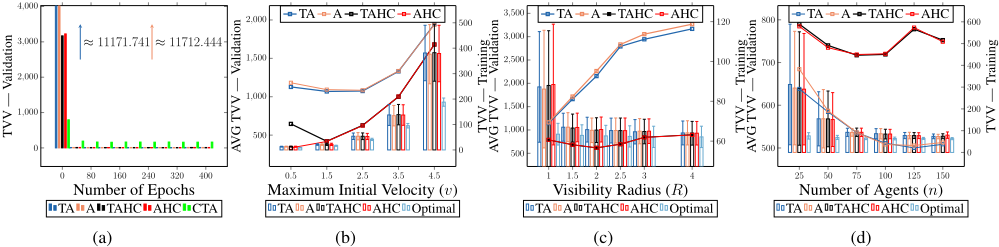
We first compare both A-GNNs and TA-GNNs to their HalfConvex counterparts and a CTA-GNN (Fig.1a). After a single epoch, our models exhibit the best performance, whereas the CTA-GNN outperforms them all. This behaviour is attributed to the fact that A-GNNs and TA-GNNs are trained by solving a non-convex ERM, which is an NP-hard process. However, during the upcoming epochs, the CTA-GNN is outperformed by all the other models, which can be explained by Theorem 1. We also note that the HC-GNNs achieve performance competitive with the non-convex GNNs. This stems from the magnified representation power attained when utilizing a linear combination of a GNN and its convex counterpart: the GNN ensures that robots approach a perfect velocity consensus, whereas the convexified GNN provides us with a faster convergence.

We now provide a comparison in regard with different flocking scenarios, which are displayed by different initial conditions. Figs.1b-1d depict the change in the average total velocity variation over the validation set and the total velocity variation over the training set (bar charts), with respect to varied values of: v (1b), R (1c), and n (1d). More accurately, in each scenario, we fix the parameters of the baseline scenario, and solely alter the examined one. We observe that the performance of all models over the training set is comparable, a fact which was also illustrated by Fig.1a. However, Figs.1b-1c illustrate that the HC-GNNs yield the best performance (on average), when regarding the validation set. This is due to the fast convergence rate during the first epoch demonstrated by Fig.1a. Yet, Fig.1d provides us with an opposite outcome: the non-convex GNNs perform better with respect to the validation set (on average). We note that this stems from the drawback embedded in convexified GNNs, which is proven by Theorem 1. Namely, since the expected generalization error is bounded by a term which depends on the number of robots n, we conclude that the higher the value of n, the higher the expected generalization error.

9 Conclusions and FutureWork

In this paper we presented convexified GNN architectures, which address the NP-hardness of common non-convex ERM problems. The proposed convex relaxation is two-fold: the nuclear norm for the rank constraint of the parameter matrix, and the RKHS relaxation for handling non-linearity. Exploiting the resulting convexity, we employed a distributed online learning scheme, so as to learn distributed controls for controlling a robotic swarm in dynamic settings.

In many real-world applications, data can be naturally represented as graphs (e.g., recommendation systems [Gao et al., 2020]), making our proposed models suitable in such contexts as well. Future work thus warrants exploring applicability of our models outside the realm of swarm robotics.

Acknowledgments

This research was funded in part by ISF grant 2306/18.