
T-SMOTE: Temporal-oriented Synthetic Minority Oversampling Technique for Imbalanced Time Series Classification
Proceedings of the Thirty-First International Joint Conference on Artificial Intelligence. Main Track. Pages 2406-2412.
https://doi.org/10.24963/ijcai.2022/334
Keywords
- Data Mining: Class Imbalance and Unequal Cost
- Data Mining: Mining Spatial and/or Temporal Data
Abstract
Time series classification is a popular and important topic in machine learning, and it suffers from the class imbalance problem in many real-world applications. In this paper, to address the class imbalance problem, we propose a novel and practical oversampling method named T-SMOTE, which can make full use of the temporal information of time-series data. In particular, for each sample of minority class, T-SMOTE generates multiple samples that are close to class border. Then, based on those samples near class border, T-SMOTE synthesizes more samples. Finally, a weighted sampling method is called on both generated samples near class border and synthetic samples. Extensive experiments on a diverse set of both univariate and multivariate time-series datasets demonstrate that T-SMOTE consistently outperforms the current state-of-the-art methods on imbalanced time series classification. More encouragingly, our empirical evaluations show that T-SMOTE performs better in the scenario of early prediction, an important application scenario in industry, which indicates that T-SMOTE could bring benefits in practice.
- [Barua et al., 2014] Sukarna Barua, Md. Monirul Islam, Xin Yao, and Kazuyuki Murase. Mwmote-majority weighted minority oversampling technique for imbalanced data set learning. IEEE Transactions on Knowledge and Data En- gineering, 26(2):405-425, 2014.
- [Bhattacharya et al., 2017] Sakyajit Bhattacharya, Vaibhav Rajan, and Harsh Shrivastava. ICU mortality prediction: A classification algorithm for imbalanced datasets. In Pro- ceedings of AAAI 2017, pages 1288-1294, 2017.
- [Bunkhumpornpat et al., 2009] Chumphol Bunkhumporn- pat, Krung Sinapiromsaran, and Chidchanok Lursinsap. Safe-Level-SMOTE: Safe-level-synthetic minority over- sampling technique for handling the class imbalanced problem. In Proceedings of PAKDD 2009, pages 475-482, 2009.
- [Cao et al., 2011] Hong Cao, Xiaoli Li, David Yew-Kwong Woon, and See-Kiong Ng. SPO: Structure preserving oversampling for imbalanced time series classification. In Proceedings of ICDM 2011, pages 1008-1013, 2011.
- [Cao et al., 2013] Hong Cao, Xiaoli Li, David Yew-Kwong Woon, and See-Kiong Ng. Integrated oversampling for imbalanced time series classification. IEEE Transactions on Knowledge and Data Engineering, 25(12):2809-2822, 2013.
- [Chawla et al., 2002] Nitesh V. Chawla, Kevin W. Bowyer, Lawrence O. Hall, and W. Philip Kegelmeyer. SMOTE: Synthetic minority over-sampling technique. Journal of Artificial Intelligence Research, 16:321-357, 2002.
- [Chi et al., 2020] Jianfeng Chi, Guanxiong Zeng, Qiwei Zhong, Ting Liang, Jinghua Feng, Xiang Ao, and Jiayu Tang. Learning to undersampling for class imbalanced credit risk forecasting. In Proceedings of ICDM 2020, pages 72-81, 2020.
- [Gong and Chen, 2016] Zhichen Gong and Huanhuan Chen. Model-based oversampling for imbalanced sequence clas- sification. In Proceedings of CIKM 2016, pages 1009- 1018, 2016.
- [Goroshin et al., 2015] Ross Goroshin, Joan Bruna, Jonathan Tompson, David Eigen, and Yann LeCun. Unsupervised learning of spatiotemporally coherent metrics. In Proceedings of ICCV 2015, pages 4086-4093, 2015.
- [Han et al., 2005] Hui Han, Wenyuan Wang, and Binghuan Mao. Borderline-SMOTE: A new over-sampling method in imbalanced data sets learning. In Proceedings of ICIC 2005, pages 878-887, 2005.
- [He and Garcia, 2009] Haibo He and Edwardo A. Garcia. Learning from imbalanced data. IEEE Transactions on Knowledge and Data Engineering, 21(9):1263-1284, 2009.
- [He et al., 2008] Haibo He, Yang Bai, Edwardo A. Garcia, and Shutao Li. ADASYN: Adaptive synthetic sampling approach for imbalanced learning. In Proceedings of IJCNN 2008, pages 1322-1328, 2008.
- [He et al., 2013] Guoliang He, Yong Duan, Tieyun Qian, and Xu Chen. Early prediction on imbalanced multivariate time series. In Proceedings of CIKM 2013, pages 1889- 1892, 2013.
- [Hochreiter and Schmidhuber, 1997] Sepp Hochreiter and Jürgen Schmidhuber. Long short-term memory. Neural Computation, 9(8):1735-1780, 1997.
- [Huang et al., 2020] Hao Huang, Chenxiao Xu, Shinjae Yoo, Weizhong Yan, Tianyi Wang, and Feng Xue. Imbalanced time series classification for flight data analyzing with nonlinear granger causality learning. In Proceedings of CIKM 2020, pages 2533-2540, 2020.
- [Jo et al., 2015] Yohan Jo, Natasha Loghmanpour, and Car- olyn Penstein Rosé. Time series analysis of nursing notes for mortality prediction via a state transition topic model. In Proceedings of CIKM 2015, pages 1171-1180, 2015.
- [Köknar-Tezel and Latecki, 2011] Suzan Köknar-Tezel and Longin Jan Latecki. Improving SVM classification on im- balanced time series data sets with ghost points. Knowl. Inf. Syst., 28(1):1-23, 2011.
- [Liang and Zhang, 2012] Guohua Liang and Chengqi Zhang. An efficient and simple under-sampling technique for imbalanced time series classification. In Proceedings of CIKM 2012, pages 2339-2342, 2012.
- [Liu and Hsieh, 2020] Chien-Liang Liu and Po-Yen Hsieh. Model-based synthetic sampling for imbalanced data. IEEE Transactions on Knowledge and Data Engineering, 32(8):1543-1556, 2020.
- [Liu et al., 2002] Bing Liu, Wee Sun Lee, Philip S. Yu, and Xiaoli Li. Partially supervised classification of text doc- uments. In Proceedings of ICML 2002, pages 387-394, 2002.
- [Luo et al., 2021] Chuan Luo, Pu Zhao, Bo Qiao, Youjiang Wu, Hongyu Zhang, Wei Wu, Weihai Lu, Yingnong Dang, Saravanakumar Rajmohan, Qingwei Lin, and Dongmei Zhang. NTAM: Neighborhood-temporal attention model for disk failure prediction in cloud platforms. In Proceed- ings of WWW 2021, pages 1181-1191, 2021.
- [Wang et al., 2015] Shuo Wang, Leandro L. Minku, and Xin Yao. Resampling-based ensemble methods for online class imbalance learning. IEEE Transactions on Knowledge and Data Engineering, 27(5):1356-1368, 2015.
- [Yan et al., 2017] Yan Yan, Tianbao Yang, Yi Yang, and Jianhui Chen. A framework of online learning with im- balanced streaming data. In Proceedings of AAAI 2017, 2017.
- [Yin et al., 2020] Jian Yin, Chunjing Gan, Kaiqi Zhao, Xuan Lin, Zhe Quan, and Zhi-Jie Wang. A novel model for im- balanced data classification. In Proceedings of AAAI 2020, pages 6680-6687, 2020.
- [Zhang et al., 2018] Chuanhai Zhang, Wallapak Ta- vanapong, Gavin Kijkul, Johnny Wong, Piet C. de Groen, and Jung-Hwan Oh. Similarity-based active learning for image classification under class imbalance. In Proceedings of ICDM 2018, pages 1422-1427, 2018.
References were extracted automatically from the PDF and may contain errors.
Full text extracted automatically from the PDF; figures, tables and equations may differ. The PDF is the version of record.
1 Introduction
Time series classification has attracted great attention since it is fundamental in machine learning. However, in many real-world applications [Chi et al., 2020; Bhattacharya et al., 2017; Wang et al., 2015; Jo et al., 2015; Goroshin et al., 2015; Zhang et al., 2018], time series classification suffers from the class imbalance problem - the number of samples from majority class is much greater than that of samples from minority class, which hinders most machine learning algorithms from achieving good performance [Liu and Hsieh, 2020].
To address the class imbalance problem, many general, practical oversampling methods have been proposed, including: Random Repetition [He and Garcia, 2009], SMOTE [Chawla et al., 2002], Borderline-SMOTE [Han et al., 2005], ADASYN [He et al., 2008], MWMOTE [Barua et al., 2014], MBS [Liu and Hsieh, 2020], etc. However, most of them do not consider the temporal information (i.e., gradually and continuously changing characteristics) of time series data, which degrades their performance. SPO [Cao et al., 2011], INOS [Cao et al., 2013] and MBO [Gong and Chen, 2016] are specific oversampling methods for handling time-series data. However, SPO and INOS can only be applied on univariate time series data, while MBO loses the sequential structure of newly-generated samples.
∗Chuan Luo is the corresponding author of this work (Email: chuanluophd@outlook.com).
Further, in many real-world scenarios of time series classification, early prediction is desirable [He et al., 2013]. Specifically, given a time series, the task of early prediction is to conduct forecasting based on the prefix sub-time series rather than taking the whole time series as input. In industrial practice, early prediction is important; for instance, in the application scenario of failure prediction in cloud platforms, hardware failures are required to be predicted as early as possible, so that proactive actions could be taken in time to mitigate negative consequences [Luo et al., 2021].
In this paper, a novel, temporal-oriented oversampling approach, dubbed T-SMOTE, is proposed for synthesizing samples for minority class. First, we consider the nature of classification that the samples, which are closer to class border, may contribute more than other samples, which are far away from class border [Han et al., 2005]. Also, considering that the nature of time series data is gradually and continuously changing, T-SMOTE generates candidate samples near class border based on the temporal characteristics of each sample in minority class, and the newly generated candidates would bring more pattern information. Then, for each generated sample x near class border, in order to incorporate temporal information, T-SMOTE utilizes a new method to determine x's neighbor based on temporal characteristics, instead of using the conventional K-Nearest-Neighbors (KNN) method adopted by existing methods; after determining x's neighbor based on temporal characteristics, T-SMOTE synthesizes more samples based x and x's neighbor. Finally, T-SMOTE employs a weighted sampling method on all generated samples near class border and all synthetic samples to mitigate the sample noise. In this way, compared to existing methods, T-SMOTE can better capture the temporal nature, and also T-SMOTE handles class imbalance problem more effectively and achieves higher performance in early prediction. We summarize the main contributions as follows:
- We propose a novel and effective oversampling method dubbed T-SMOTE for imbalanced time series classification. In order to handle the class imbalance problem on time series data effectively, T-SMOTE aims to generate more samples near class border for minority class.
- T-SMOTE proposes to utilize a new method to synthesize more samples for minority class based on temporal characteristics, compared to existing methods that adopt conventional KNN method.
- We conduct extensive experiments on both univariate and multivariate datasets to compare T-SMOTE against 8 state-of-the-art competitors, and the results show that T-SMOTE better handles class imbalance problem on both univariate time series data and multivariate time series data. Further, our evaluations present that T-SMOTE can achieve better performance in early prediction.
2 Our Proposed T-SMOTE Approach
In this section, we present the technical details of our proposed T-SMOTE approach.
2.1 Preliminaries
Following the common practice without loss of generality, we treat the minority class as positive class and the majority class as negative class. Therefore, in the context of imbalanced time series classification, the number of positive samples is much less than the the number of negative samples. The goal of our method is to re-balance the training set by generating more positive synthetic samples, in order to achieve better performance in the subsequent classification task.
For simplicity, we denote the set of raw positive samples in training set as P = {X1, . . . ,Xi, . . . ,Xn}, where Xi is a positive sample with feature values collected at all timestamps. Positive sample Xi = (x1i · · · xTi ) ∈ RT×d is a 2-dimensional matrix consisting of a series of feature vectors, where T is the last timestamp and also indicates the sequence length. For timestamp j ∈ {1, . . . , T}, feature vector xji ∈ Rd is a 1-dimensional vector with d feature values collected at j-th timestamp. Notation N denotes the set of all negative samples in training set, and the imbalance ratio is r = |N|/|P |.
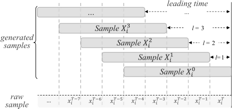
For each raw sample Xi, we generate new samples based on subsequences [He et al., 2013] with length w. As illustrated in Figure 1, a generated sample Xl i =
(xT -l-w+1 i , · · · , xT-l i ) is a subsequence of Xi with length w and the last timestamp of T - l, where l is the leading time of the generated sample. Given a specific leading time l, Xl = {Xl1 , . . . ,X l i , . . . ,X ln } is the set of all generated samples for raw samples in X.
2.2 Approach Overview
Our proposed T-SMOTE approach consists of three steps: (1) based on each positive sample, T-SMOTE generates a set of candidate samples near class border; (2) for each generated sample x near class border, T-SMOTE synthesizes more samples considering x's temporal characteristics; (3) T-SMOTE employs a weighted sampling method on all generated samples, in order to alleviate sample noise.
2.3 Generation of Near-border Samples
In the research field of machine learning, since the classification task aims to determine a class border between different classes, it is intuitive that near-border samples (i.e., samples near class border) would contribute more to the classification task than those far away from class border [Han et al., 2005]. For oversampling methods, the common practice of seeking near-border samples is based on KNN algorithm. However, conventional KNN algorithm is unsuitable for handling 2-dimensional time-series data [K¨oknar-Tezel and Latecki, 2011]. In fact, considering the gradually and continuously changing characteristics of time series data, compared to Xl i , sample Xl+1 i (with larger leading time) is closer to class border. Further, it is intuitive that, if the leading time l is too large-valued, then the corresponding sample with such large leading time would possibly belong to negative class. For example, in the scenario of hardware failure prediction (where positive and negative samples correspond to failure and health, respectively), a sample with larger leading time means that the corresponding timestamp is farther away from failure occurrence, so the hardware at the corresponding timestamp tends to be healthy.
Hence, for each raw positive sample Xi, the process of generating new near-border samples underlying T-SMOTE is illustrated in Figure 1. From Figure 1, T-SMOTE generates multiple samples X0 i ,X1 i , . . . ,X L i sequentially. As discussed before, with the increment of leading time, such generated samples with larger leading time would be closer to class border. Through this way, T-SMOTE can generate (L + 1) × |P | positive samples in total.
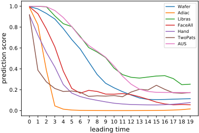
Furthermore, to verify the aforementioned intuition that the positive samples with larger leading time are closer to class border, we conduct empirical studies. It is recognized that the prediction score of positive samples tends to be 1, while the prediction score of negative samples tends to be 0; thus, if the intuition is reasonable, the prediction score of generated samples with larger leading time should be smaller (even around 0), since samples with enough large leading time would belong to negative class. In our empirical study, we first train a long short-term memory (LSTM) model [Hochreiter and Schmidhuber, 1997] based on various raw training sets, and then use such trained LSTM model to predict the generated samples with various leading time. Figure 2 presents the average prediction score output by our trained LSTM model with different leading time on various datasets (which will be described in the Experiments section). According to Figure 2, the prediction score decreases with the increment of leading time, which verifies our intuition.
Then, we need to address how to decide the maximum leading time L that not only makes the generated samples near class border but also makes the samples possibly belong to positive class. To address this problem, we employ a spy-based method, which has shown success in the field of positive-unlabeled learning to identify true negative samples from unlabeled data [Liu et al., 2002]. Following the standard practice [Liu et al., 2002], we randomly select 15% of negative samples and relabel them to positive to act as spies Pspy and mix them with positive samples P , resulting in a new set of spy-injected positive samples P ′ = P ∪ Pspy and a new set of negative samples N ′ = N-Pspy. Then, we re-balance the P ′ and N ′ by randomly repeating [He and Garcia, 2009] the true positive samples in P ′ , and train a classifier f based on the balanced P ′ and N ′ . Afterwards, we can obtain prediction scores of all spy samples Pspy based on f, and set the maximum score as threshold h. Finally, we iteratively generate samples Xl with leading time of l (l increases from 0): in the iteration where l = l0, if the average prediction score Sl0 = Σni=0 f (Xl0 i )/n of Xl0 is smaller than threshold h, T-SMOTE considers that Xl0 belongs to negative class and should be neglected; meanwhile, the process of generating near-border samples is terminated. Hence, we obtain L = l0 - 1, and all generated samples with leading time no greater than L are regarded as positive ones.
After the generation of near-border samples, we can obtain L+ 1 generated positive samples for each Xi, and each sample has a related prediction score sli = f(Xl i ), resulting in a sample-score pair (Xl i , sli ), where sli indicates the probability of Xl i that belongs to positive class.
2.4 Generation of More Synthetic Samples
In traditional SMOTE method and its variants, the key process is to find a suitable neighbor for each positive sample and then generate a synthetic sample along the line segment between this positive sample and its neighbor. In our approach, we follow this direction, but propose a new method to synthesize more samples for minority class regarding temporal characteristics. Compared to SMOTE that calculates the Euclidean distance between the feature vectors to find the knearest neighbors, T-SMOTE defines a novel concept of temporal neighbor as follows: for each positive sample Xl i with leading time l, Xl i and Xl+1 i are temporal neighbors. In particular, T-SMOTE uses temporal neighbor to exploit the temporal characteristics of time series data. In more detail, for sample Xl i , T-SMOTE synthesizes more samples along the line segment between Xl i and its temporal neighbor Xl+1 i :
where α is a random value generated by Beta distribution B(sli , sl+1 i ), which is a continuous probability distributions defined on the interval [0, 1] and is the conjugate prior probability distribution for the Bernoulli distribution. The reason why T-SMOTE does not use Gaussian Distribution as other works do is that T-SMOTE can make full use of the prior knowledge. Besides, if a feature is categorical, T-SMOTE selects the specific value from Xl i with the probability of α (i.e., selecting the specific value from Xl+1 i with probability of 1 - α) as the new feature value. The score of the newly synthetic Xnew is as follows:
Then, we need to address how many synthetic samples should be generated for each Xl i . Inspired by safe-levelSMOTE and ADASYN, the number of synthetic samples should be decided based on the safe level of Xl i . In practice, if the prediction score of Xl i is larger, then Xl i is with higher safe level. Hence, it is advisable to synthesize more samples with regard to higher safe level. Specifically, T-SMOTE determines the number of synthetic samples as follows:
where r is the imbalance ratio (as defined in Section 2.1). Afterwards, we can obtain mli synthetic, positive samples based on each Xl i . Also, each synthetic sample has a related score to indicate the probability to be positive.
2.5 Weighted SamplingMethod
As mentioned in [Bunkhumpornpat et al., 2009; Liu and Hsieh, 2020], the samples near class border may lead to an ambiguous situation. To address this issue, T-SMOTE utilizes a weighted sampling method to reduce the risk from nearborder samples. For each sample X, we first assign to X a weight w = max(0, s - h), where s is the prediction score of X, and h is the threshold determined in the generation of near-border samples. Finally, T-SMOTE constructs the final positive dataset P ′ by randomly selecting |N| samples from all generated positive samples with the selection probability that is proportional to the each sample's weight w.
3 Experiments
In this section, to demonstrate the effectiveness of T-SMOTE, we conduct extensive experiments on 7 public univariate and 3 multivariate time-series datasets to compare T-SMOTE against 8 state-of-the-art competitors.
| Dataset | Dimensions | #Class | #Sample | Positive class | #Pos | Imbalance ratio | Time series length | |
|---|---|---|---|---|---|---|---|---|
| multivariate | Libras | 2 | 15 | 360 | 7 | 24 | 14.00 | 45 |
| Hand | 3 | 20 | 2858 | 1 | 171 | 15.70 | [60,182] | |
| AUS | 22 | 95 | 2565 | crazy | 27 | 94.00 | [45,136] | |
| 50Words | 1 | 50 | 450 | 4 | 20 | 21.5 | 270 | |
| Adiac | 1 | 37 | 390 | 25 | 10 | 37.70 | 176 | |
| FaceAll | 1 | 14 | 560 | 10 | 40 | 13.00 | 131 | |
| univariate SLeaf | 1 | 15 | 500 | 10 | 25 | 18.96 | 128 | |
| TwoPats | 1 | 4 | 1000 | 4 | 50 | 15.16 | 128 | |
| Wafer | 1 | 2 | 1000 | -1 | 50 | 18.06 | 152 | |
| Yoga | 1 | 2 | 300 | 1 | 15 | 10.87 | 426 |
MBO are proposed specifically for time series data: MBO can handle multivariate time-series data by default; Since original INOS is only designed for univariate time series data, to address this problem, for INOS we treat each multivariate sample as multiple univariate samples and process them separately. Besides INOS and MBO, other competitors can only accept 1-dimensional vector as input, while time series samples are 2-dimensional matrix which contains both timestamp and feature dimensions. In our experiments, we concatenate the raw 2-dimensional sample along the timestamp dimension to flatten the matrix as 1-dimensional vector for these competitors that only accept 1-dimensional vector.
3.3 Experimental Setup
Evaluation Metrics
We adopt three widely used metrics in imbalance learning to evaluate the performance of each approach, including (1) AUC, the Area Under the ROC Curve, which used in [Gong and Chen, 2016; Yan et al., 2017; Yin et al., 2020; Barua et al., 2014]; (2) F1: a general metric in classification as adopted by [Cao et al., 2013; Gong and Chen, 2016; Liu and Hsieh, 2020; Liang and Zhang, 2012; Cao et al., 2011; Yin et al., 2020; Barua et al., 2014]; (3) AUPRC: the Area Under the Precision-Recall Curve, a useful performance indicator for imbalanced data in the scenarios focusing finding positive samples, as used in [Huang et al., 2020; Yan et al., 2017].
Classifier Specification
In our experiments, after getting the re-balanced training datasets generated by T-SMOTE and all its competitors, we employ a uniform classifier to evaluate the quality of the generated datasets. In particular, in our experiments we adopt
3.1 Datasets
There are ten datasets that are commonly used in the context of imbalanced time-series classification [Cao et al., 2011; Cao et al., 2013; Gong and Chen, 2016]: (1) seven univariate datasets from UCR 1 time series repository, including Adiac, 50Words, FaceAll, SLeaf, TwoPats, Wafer and Yoga; (2) three multivariate datasets fromUCI 2 time series repository, including Libras, Hand and AUS. Following the common preprocessing practices in [Cao et al., 2013] and [Gong and Chen, 2016]: as these datasets originally contain multiple classes, we convert them into two-class by randomly selecting one class as the positive class and treat the rest classes as the negative class. Additionally, in order to create high imbalance ratio and simulate the scenario of rare positive instances, we randomly select partial samples from the positive class and abandon others. For the split of training set and testing set, we randomly select 70% as training set and 30% as testing for each multivariate dataset in UCI following [Gong and Chen, 2016]; as these univariate datasets from UCR contain both training set and testing set, no extra processing is required. A summary of the datasets in our experiments is reported in Table 1.
3.2 Competitors
To evaluate T-SMOTE, we compare T-SMOTE with eight widely used, state-of-the-art competitors, including Repeat [He and Garcia, 2009], B-SMOTE [Chawla et al., 2002], ADASYN [He et al., 2008], MWMOTE [Barua et al., 2014], MBS [Liu and Hsieh, 2020], INOS [Cao et al., 2013] and MBO [Gong and Chen, 2016]. Among them, INOS and LSTM [Hochreiter and Schmidhuber, 1997] as the uniform classifier, since LSTM is recognized to be a commonly-used and effective time series prediction model.
1 http://www.cs.ucr.edu/∼eamonn/time series data
2 https://archive.ics.uci.edu/ml/datasets.php
| Dataset | Repeat | SMOTE | B-SMOTE | ADASYN | MWMOTE | MBS | INOS | MBO | T-SMOTE |
|---|---|---|---|---|---|---|---|---|---|
| 50Words | 0.8422 | 0.8635 | 0.8513 | 0.8608 | 0.8605 | 0.8665 | 0.8726 | 0.8747 | 0.8926 |
| Adiac | 0.9453 | 0.9500 | 0.9603 | 0.9618 | 0.9630 | 0.9718 | 0.9815 | 0.9803 | 0.9926 |
| FaceAll | 0.9468 | 0.9510 | 0.9535 | 0.9573 | 0.9519 | 0.9554 | 0.9684 | 0.9677 | 0.9858 |
| Sleaf | 0.9295 | 0.9584 | 0.9720 | 0.9708 | 0.9656 | 0.9729 | 0.9767 | 0.9823 | 0.9987 |
| AUC TwoPats | 0.8731 | 0.8833 | 0.8877 | 0.8932 | 0.8839 | 0.8967 | 0.9077 | 0.9096 | 0.9130 |
| Wafer | 0.9629 | 0.9782 | 0.9760 | 0.9755 | 0.9691 | 0.9793 | 0.9890 | 0.9888 | 0.9992 |
| Yoga | 0.6526 | 0.6667 | 0.6712 | 0.6710 | 0.6624 | 0.6870 | 0.6973 | 0.7116 | 0.7228 |
| Libras | 0.9138 | 0.9612 | 0.9585 | 0.9663 | 0.9513 | 0.9715 | 0.9838 | 0.9905 | 0.9975 |
| Hand | 0.9266 | 0.9367 | 0.9334 | 0.9394 | 0.9469 | 0.9456 | 0.9504 | 0.9585 | 0.9751 |
| AUS | 0.9684 | 0.9723 | 0.9796 | 0.9804 | 0.9719 | 0.9801 | 0.9889 | 0.9887 | 0.9991 |
| average | 0.8961 | 0.9121 | 0.9143 | 0.9177 | 0.9126 | 0.9227 | 0.9316 | 0.9353 | 0.9476 |
| 50Words | 0.5227 | 0.5455 | 0.5412 | 0.5376 | 0.5614 | 0.5588 | 0.5714 | 0.5803 | 0.5946 |
| Adiac | 0.6364 | 0.6522 | 0.6767 | 0.6809 | 0.6879 | 0.7011 | 0.7468 | 0.7500 | 0.7692 |
| FaceAll | 0.7347 | 0.7395 | 0.7511 | 0.7542 | 0.7373 | 0.7699 | 0.7982 | 0.8013 | 0.8367 |
| Sleaf | 0.8624 | 0.9000 | 0.9107 | 0.9131 | 0.9193 | 0.9207 | 0.9320 | 0.9288 | 0.9484 |
| F1 TwoPats | 0.6451 | 0.6521 | 0.6531 | 0.6502 | 0.6536 | 0.6603 | 0.6716 | 0.6705 | 0.6826 |
| Wafer | 0.9349 | 0.9456 | 0.9497 | 0.9515 | 0.9562 | 0.9553 | 0.9603 | 0.9641 | 0.9756 |
| Yoga | 0.5688 | 0.6033 | 0.6062 | 0.5859 | 0.5907 | 0.6068 | 0.6165 | 0.6189 | 0.6273 |
| Libras | 0.7967 | 0.8571 | 0.8392 | 0.8489 | 0.8300 | 0.8571 | 0.8889 | 0.9333 | 0.9333 |
| Hand | 0.5366 | 0.5655 | 0.5593 | 0.5634 | 0.5854 | 0.5855 | 0.6000 | 0.6087 | 0.6202 |
| AUS | 0.6250 | 0.6667 | 0.7059 | 0.7143 | 0.7273 | 0.7500 | 0.7692 | 0.8000 | 0.8333 |
| average | 0.6863 | 0.7127 | 0.7193 | 0.7200 | 0.7249 | 0.7365 | 0.7555 | 0.7656 | 0.7821 |
| 50Words | 0.5341 | 0.5430 | 0.5522 | 0.5375 | 0.5600 | 0.5516 | 0.5723 | 0.5743 | 0.5903 |
| Adiac | 0.8694 | 0.8701 | 0.8777 | 0.8754 | 0.8809 | 0.8836 | 0.8992 | 0.8970 | 0.9202 |
| FaceAll | 0.8771 | 0.8839 | 0.9047 | 0.9084 | 0.8904 | 0.9111 | 0.9210 | 0.9202 | 0.9365 |
| Sleaf | 0.9440 | 0.9535 | 0.9532 | 0.9608 | 0.9601 | 0.9632 | 0.9703 | 0.9712 | 0.9886 |
| AUPRC TwoPats | 0.6796 | 0.7016 | 0.7048 | 0.7175 | 0.7104 | 0.7136 | 0.7310 | 0.7264 | 0.7487 |
| Wafer | 0.9318 | 0.9461 | 0.9507 | 0.9488 | 0.9525 | 0.9548 | 0.9669 | 0.9680 | 0.9885 |
| Yoga | 0.6594 | 0.6667 | 0.6807 | 0.6765 | 0.6825 | 0.6906 | 0.7050 | 0.7019 | 0.7154 |
| Libras | 0.8612 | 0.8817 | 0.8760 | 0.8915 | 0.8764 | 0.9184 | 0.9427 | 0.9526 | 0.9750 |
| Hand | 0.6776 | 0.6852 | 0.6803 | 0.6789 | 0.6880 | 0.6917 | 0.7003 | 0.7033 | 0.7101 |
| AUS | 0.8445 | 0.8769 | 0.8782 | 0.8839 | 0.8810 | 0.8929 | 0.9004 | 0.9095 | 0.9214 |
| average | 0.7879 | 0.8009 | 0.8059 | 0.8079 | 0.8082 | 0.8172 | 0.8309 | 0.8324 | 0.8495 |
3.4 Experimental Results on All Dataset
Table 2 shows the comparative results of T-SMOTE and its 8 competitors on both 7 univariate and 3 multivariate datasets. For each dataset, the best results across all 9 methods are indicated in boldface. It is clear that T-SMOTE achieves the best or equal best performance across all metrics of F1, AUPRC, and AUC compared to all its competitors on both univariate and multivariate datasets.
In particular, on univariate datasets, in terms of F1, AUPRC and AUC, T-SMOTE achieves average values of 0.7763, 0.8412 and 0.9293, which are considerably higher than those achieved by all its competitors. Compared to the second best method MBO with the average AUC value of 0.9164, T-SMOTE achieves 3.10% improvement, which is substantial considering high AUC values achieved by baseline competitors. Besides, on the multivariate datasets, the average F1, AUPRC and AUC values achieved by T-SMOTE are 0.7956, 0.8688 and 0.9906, and T-SMOTE performs much better than all its competitors. In terms of the evaluation metric of AUC, T-SMOTE outperforms the second best method MBO with a relative improvement of 2.36%. Specifically, on dataset AUS, T-SMOTE yields the F1 value of 0.8333, which is 3.33% higher than MBO. Therefore, the results in Table 2 clearly demonstrate the superiority of T- SMOTE over all its competitors on both univariate and multivariate datasets, which indicates that T-SMOTE might be able to bring benefits in practice.
3.5 Effectiveness of Using Temporal Information
To demonstrate the advantage of considering the temporal information, we further analyze the results in Table 2. As aforementioned, INOS, MBO and T-SMOTE are all designed to utilize temporal information, while other methods are not.
According to Table 2, it is apparent that, on all evaluation metrics of AUC, F1 and AUPRC, those methods that capture temporal information (i.e., INOS, MBO and T-SMOTE) achieve much better performance than other methods that do not utilize temporal information. Specifically, T-SMOTE is a variant of B-SMOTE and fully incorporates temporal information. When directly comparing T-SMOTE and B-SMOTE, the AUC, F1, AUPRC values achieved by T-SMOTE are 0.9476, 0.7821 and 0.8495, respectively, while those values obtained by B-SMOTE are 0.9143, 0.7193 and 0.8059, respectively. Hence, the performance improvement achieved by T-SMOTE is substantial. The observation confirms the considerable contribution of making the use of temporal information in both univariate and multivariate time series classification tasks.
3.6 Experimental Results of Early Prediction
We conduct experiments to demonstrate that the adoption of generating samples with larger leading time is able to help T-SMOTE achieve better early prediction performance. The testing dataset is constructed as follows: for each testing dataset, the positive samples are generated using the specific leading times of l = 3, l = 5, l = 10 separately (for example, l = 5 means we conduct prediction ahead of 5 timestamps). Then we test the performance of each method on testing dataset, and the related results are reported in Table 3.
| Leading time = 3 | Leading time = 5 | Leading time = 10 | |||||||
|---|---|---|---|---|---|---|---|---|---|
| Dataset | INOS | MBO | T-SMOTE | INOS | MBO | T-SMOTE | INOS | MBO | T-SMOTE |
| 50Words | 0.8487 | 0.8527 | 0.8820 | 0.7968 | 0.7891 | 0.8457 | 0.7674 | 0.7773 | 0.8394 |
| Adiac | 0.9373 | 0.9543 | 0.9823 | 0.8523 | 0.8785 | 0.9367 | 0.7230 | 0.7472 | 0.8330 |
| FaceAll | 0.9625 | 0.9651 | 0.9818 | 0.9294 | 0.9325 | 0.9430 | 0.5488 | 0.5263 | 0.7203 |
| Sleaf | 0.9708 | 0.9820 | 0.9978 | 0.9664 | 0.9788 | 0.9972 | 0.9574 | 0.9643 | 0.9935 |
| AUC TwoPats | 0.8697 | 0.8869 | 0.9045 | 0.8291 | 0.8356 | 0.8869 | 0.7329 | 0.7481 | 0.7923 |
| Wafer | 0.9828 | 0.9830 | 0.9986 | 0.9376 | 0.9392 | 0.9721 | 0.8069 | 0.8023 | 0.8316 |
| Yoga | 0.6917 | 0.6976 | 0.7136 | 0.6382 | 0.6456 | 0.6880 | 0.5794 | 0.5912 | 0.6632 |
| Libras | 0.9775 | 0.9895 | 0.9962 | 0.9662 | 0.9738 | 0.9913 | 0.8375 | 0.8737 | 0.9487 |
| Hand | 0.9589 | 0.9606 | 0.9701 | 0.8700 | 0.8940 | 0.9231 | 0.5209 | 0.5744 | 0.7621 |
| AUS | 0.9721 | 0.9765 | 0.9976 | 0.9645 | 0.9649 | 0.9951 | 0.9268 | 0.9337 | 0.9604 |
| average | 0.9172 | 0.9248 | 0.9425 | 0.8751 | 0.8832 | 0.9179 | 0.7401 | 0.7539 | 0.8345 |
| 50Words | 0.5455 | 0.5507 | 0.5714 | 0.4848 | 0.4938 | 0.5352 | 0.4375 | 0.4561 | 0.5111 |
| Adiac | 0.6522 | 0.6818 | 0.7317 | 0.5238 | 0.5660 | 0.6512 | - | - | - |
| FaceAll | 0.7670 | 0.7735 | 0.8190 | 0.6254 | 0.6408 | 0.6992 | 0.0368 | 0.0685 | 0.1714 |
| Sleaf | 0.9011 | 0.9149 | 0.9412 | 0.8750 | 0.8980 | 0.9375 | 0.7778 | 0.8193 | 0.9263 |
| F1 TwoPats | 0.6273 | 0.6407 | 0.6672 | 0.5574 | 0.5713 | 0.6234 | 0.4199 | 0.4106 | 0.5080 |
| Wafer | 0.9262 | 0.9347 | 0.9556 | 0.8319 | 0.8429 | 0.8988 | 0.3499 | 0.3438 | 0.4425 |
| Yoga | 0.5844 | 0.6006 | 0.6200 | 0.5482 | 0.5368 | 0.5856 | 0.4683 | 0.4894 | 0.5514 |
| Libras | 0.7692 | 0.8000 | 0.8517 | 0.6667 | 0.7059 | 0.7778 | 0.4000 | 0.4286 | 0.5455 |
| Hand | 0.5455 | 0.5660 | 0.6055 | 0.3333 | 0.3646 | 0.4646 | - | - | 0.0513 |
| AUS | 0.7692 | 0.8000 | 0.8333 | 0.7500 | 0.7614 | 0.8333 | 0.6087 | 0.6250 | 0.7273 |
| average | 0.7088 | 0.7263 | 0.7597 | 0.6197 | 0.6382 | 0.7007 | 0.3499 | 0.3641 | 0.4435 |
| 50Words | 0.5455 | 0.5498 | 0.5606 | 0.4943 | 0.5152 | 0.5422 | 0.4262 | 0.4333 | 0.5135 |
| Adiac | 0.8347 | 0.8400 | 0.8839 | 0.7145 | 0.7204 | 0.8010 | 0.1240 | 0.1364 | 0.3785 |
| FaceAll | 0.8156 | 0.8264 | 0.8796 | 0.6570 | 0.7181 | 0.7809 | 0.0572 | 0.0642 | 0.1615 |
| Sleaf | 0.9678 | 0.9644 | 0.9826 | 0.9339 | 0.9402 | 0.9767 | 0.8929 | 0.9176 | 0.9632 |
| AUPRC TwoPats | 0.6231 | 0.6978 | 0.7222 | 0.5975 | 0.6168 | 0.6546 | 0.5167 | 0.5139 | 0.5766 |
| Wafer | 0.9666 | 0.9633 | 0.9802 | 0.8654 | 0.8800 | 0.9283 | 0.5021 | 0.5014 | 0.6434 |
| Yoga | 0.6791 | 0.6874 | 0.7075 | 0.6008 | 0.6278 | 0.6664 | 0.5917 | 0.5980 | 0.6367 |
| Libras | 0.8795 | 0.8998 | 0.9526 | 0.8242 | 0.8495 | 0.9184 | 0.5765 | 0.6029 | 0.7441 |
| Hand | 0.6337 | 0.6424 | 0.7072 | 0.2096 | 0.3341 | 0.4712 | 0.0393 | 0.0414 | 0.1435 |
| AUS | 0.8716 | 0.8901 | 0.9137 | 0.8307 | 0.8562 | 0.9047 | 0.7082 | 0.7250 | 0.8269 |
| average | 0.7817 | 0.7961 | 0.8290 | 0.6728 | 0.7058 | 0.7644 | 0.4435 | 0.4534 | 0.5588 |
The results presented in Table 3 clearly demonstrates that T-SMOTE achieves the best performance under all leading time, and its advantage becomes greater with the increment of leading time. For example, the average value of AUPRC achieved by T-SMOTE is 0.8290, which is 3.29% greater than the second best competitor MBO when the leading time is 3, and the performance improvement becomes 5.86% when leading time is 5. Furthermore, when leading time is 10, T-SMOTE outperforms MBO by 10.54%. This is intuitive, because the samples generated by T-SMOTE contains those ones with different leading times, which make the classifier learn more informative patterns and thus drive T-SMOTE outperform its competitors.
Also, from Table 3, with the increment of l from 3 to 10, the values of F1, AUPUR and AUC obtained by all oversampling methods degrade. Specifically, on the Adiac dataset, when leading time is 10, the F1 values achieved by INOS, MBO and T-SMOTE all drop to 0, which means that the classifiers trained with INOS, MBO and T-SMOTE fail to predict ahead of 10 timestamps. Actually, this is not surprising since samples with larger leading time are closer to or even across the class border from the positive class side to the negative class side, resulting in great class noise for the classifier.
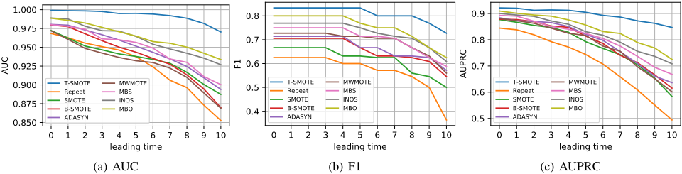
To further study the effect between classification performance and leading time, we randomly select the AUS dataset to analyze their relationship. According to Figure 3, all methods suffer from the performance degradation with the increment of leading time. However, for any specific increment leading time, T-SMOTE still achieves the best performance. Besides, it is apparent that those methods that capture temporal information (i.e., T-SMOTE, INOS and MBO) always outperform other methods on various values of leading time.
4 Conclusions
Imbalanced time series classification is a popular and practical topic in diverse real-world applications. In this paper, we propose a novel temporal-oriented oversampling method dubbed T-SMOTE which considers the gradually and continuously changing characteristics in time-series datasets. T-SMOTE can process both univariate and multivariate datasets, and it can also perform well in the scenario of early prediction. Our extensive experiments on 10 datasets demonstrate that T-SMOTE achieves significantly better performance than all its state-of-the-art competitors. Moreover, T-SMOTE has been deployed to several scenarios in Microsoft Azure and Microsoft 365, such as disk failure prediction and high latency prediction, and has considerably improved the performance of the online models.
@inproceedings{ijcai2022p334,
  title     = {T-SMOTE: Temporal-oriented Synthetic Minority Oversampling Technique for Imbalanced Time Series Classification},
  author    = {Zhao, Pu and Luo, Chuan and Qiao, Bo and Wang, Lu and Rajmohan, Saravan and Lin, Qingwei and Zhang, Dongmei},
  booktitle = {Proceedings of the Thirty-First International Joint Conference on
               Artificial Intelligence, {IJCAI-22}},
  publisher = {International Joint Conferences on Artificial Intelligence Organization},
  editor    = {Luc De Raedt},
  pages     = {2406--2412},
  year      = {2022},
  month     = {7},
  note      = {Main Track},
  doi       = {10.24963/ijcai.2022/334},
  url       = {https://doi.org/10.24963/ijcai.2022/334},
}
TY - CPAPER TI - T-SMOTE: Temporal-oriented Synthetic Minority Oversampling Technique for Imbalanced Time Series Classification AU - Zhao, Pu AU - Luo, Chuan AU - Qiao, Bo AU - Wang, Lu AU - Rajmohan, Saravan AU - Lin, Qingwei AU - Zhang, Dongmei T2 - Proceedings of the Thirty-First International Joint Conference on Artificial Intelligence, IJCAI-22 PB - International Joint Conferences on Artificial Intelligence Organization PY - 2022 SP - 2406 EP - 2412 DO - 10.24963/ijcai.2022/334 UR - https://doi.org/10.24963/ijcai.2022/334 ER -Copied
Machine-readable versions of this paper, for tools and AI agents:





