
Self-Supervised Mutual Learning for Dynamic Scene Reconstruction of Spiking Camera
Proceedings of the Thirty-First International Joint Conference on Artificial Intelligence. Main Track. Pages 2859-2866.
https://doi.org/10.24963/ijcai.2022/396
Keywords
- Machine Learning: Unsupervised Learning
- Machine Learning: Self-supervised Learning
Abstract
Mimicking the sampling mechanism of the primate fovea, a retina-inspired vision sensor named spiking camera has been developed, which has shown great potential for capturing high-speed dynamic scenes with a sampling rate of 40,000 Hz. Unlike conventional digital cameras, the spiking camera continuously captures photons and outputs asynchronous binary spikes with various inter-spike intervals to record dynamic scenes. However, how to reconstruct dynamic scenes from asynchronous spike streams remains challenging. In this work, we propose a novel pretext task to build a self-supervised reconstruction framework for spiking cameras. Specifically, we utilize the blind-spot network commonly used in self-supervised denoising tasks as our backbone, and perform self-supervised learning by constructing proper pseudo-labels. In addition, in view of the poor scalability and insufficient information utilization of the blind-spot network, we present a mutual learning framework to improve the overall performance of the network through mutual distillation between a non-blind-spot network and a blind-spot network. This also enables the network to bypass constraints of the blind-spot network, allowing state-of-the-art modules to be used to further improve performance. The experimental results demonstrate that our methods evidently outperform previous unsupervised spiking camera reconstruction methods and achieve desirable results compared with supervised methods.
- [Brandli et al., 2014] Christian Brandli, Raphael Berner, Minhao Yang, Shih-Chii Liu, and Tobi Delbruck. A 240× 180 130 db 3 µs latency global shutter spatiotemporal vision sensor. IEEE Journal of Solid-State Circuits, 49(10):2333-2341, 2014.
- [Byun et al., 2021] Jaeseok Byun, Sungmin Cha, and Taesup Moon. FBI-Denoiser: Fast blind image denoiser for poisson- gaussian noise. In CVPR, pages 5768-5777, 2021.
- [Choi et al., 2020] Jonghyun Choi, Kuk-Jin Yoon, et al. Learning to super resolve intensity images from events. In CVPR, pages 2768-2776, 2020.
- [Dong et al., 2017] Siwei Dong, Tiejun Huang, and Yonghong Tian. Spike camera and its coding methods. DCC, 2017.
- [Dong et al., 2019] Siwei Dong, Lin Zhu, Daoyuan Xu, Yonghong Tian, and Tiejun Huang. An efficient coding method for spike camera using inter-spike intervals. DCC, 2019.
- [Fu et al., 2019] Jun Fu, Jing Liu, Haijie Tian, Yong Li, Yongjun Bao, Zhiwei Fang, and Hanqing Lu. Dual attention network for scene segmentation. In CVPR, pages 3146-3154, 2019.
- [Gallego et al., 2022] Guillermo Gallego, Tobi Delbrück, Garrick Orchard, Chiara Bartolozzi, Brian Taba, et al. Event-based vi- sion: A survey. IEEE Transactions on PAMI, 44(1):154-180, 2022.
- [Hinton et al., 2015] Geoffrey Hinton, Oriol Vinyals, and Jeff Dean. Distilling the knowledge in a neural network. arXiv preprint arXiv:1503.02531, 2015.
- [Huang et al., 2017] Jing Huang, Menghan Guo, and Shoushun Chen. A dynamic vision sensor with direct logarithmic output and full-frame picture-on-demand. In ISCAS, pages 1-4, 2017.
- [Huang et al., 2019] Zilong Huang, Xinggang Wang, Lichao Huang, Chang Huang, Yunchao Wei, and Wenyu Liu. Ccnet: Criss-cross attention for semantic segmentation. In ICCV, pages 603-612, 2019.
- [Huang et al., 2021] Tao Huang, Songjiang Li, Xu Jia, Huchuan Lu, and Jianzhuang Liu. Neighbor2neighbor: Self-supervised de- noising from single noisy images. In CVPR, pages 14781-14790, 2021.
- [Krull et al., 2019] Alexander Krull, Tim-Oliver Buchholz, and Florian Jug. Noise2void-learning denoising from single noisy images. In CVPR, pages 2129-2137, 2019.
- [Laine et al., 2019] Samuli Laine, Tero Karras, Jaakko Lehtinen, and Timo Aila. High-quality self-supervised deep image denois- ing. NeurIPS, 32:6970-6980, 2019.
- [Lehtinen et al., 2018] Jaakko Lehtinen, Jacob Munkberg, Jon Has- selgren, Samuli Laine, Tero Karras, Miika Aittala, and Timo Aila. Noise2noise: Learning image restoration without clean data. In ICML, pages 2971-2980, 2018.
- [Liu et al., 2019] Shih-Chii Liu, Bodo Rueckauer, Enea Ceolini, Adrian Huber, and Tobi Delbruck. Event-driven sensing for ef- ficient perception: Vision and audition algorithms. IEEE Signal Processing Magazine, 36(6):29-37, 2019.
- [Masland, 2012] Richard H Masland. The neuronal organization of the retina. Neuron, 76(2):266-280, 2012.
- [Nah et al., 2019] Seungjun Nah, Sungyong Baik, Seokil Hong, Gyeongsik Moon, Sanghyun Son, Radu Timofte, and Kyoung Mu Lee. Ntire 2019 challenge on video deblurring and super- resolution: Dataset and study. In CVPR Workshops, pages 0-0, 2019.
- [Peng et al., 2021] Rui Peng, Ronggang Wang, Yawen Lai, Luyang Tang, and Yangang Cai. Excavating the potential capacity of self- supervised monocular depth estimation. In ICCV, pages 15560- 15569, 2021.
- [Pini et al., 2018] Stefano Pini, Guido Borghi, and Roberto Vez- zani. Learn to see by events: Color frame synthesis from event and rgb cameras. arXiv preprint arXiv:1812.02041, 2018.
- [Posch et al., 2008] Christoph Posch, Daniel Matolin, and Rainer Wohlgenannt. An asynchronous time-based image sensor. In ISCAS, pages 2130-2133, 2008.
- [Rebecq et al., 2019a] Henri Rebecq, René Ranftl, Vladlen Koltun, and Davide Scaramuzza. Events-to-video: Bringing modern computer vision to event cameras. In CVPR, pages 3857-3866, 2019.
- [Rebecq et al., 2019b] Henri Rebecq, René Ranftl, Vladlen Koltun, and Davide Scaramuzza. High speed and high dynamic range video with an event camera. IEEE Transactions on PAMI, 2019.
- [Sheth et al., 2021] Dev Yashpal Sheth, Sreyas Mohan, Joshua L Vincent, Ramon Manzorro, Peter A Crozier, Mitesh M Khapra, Eero P Simoncelli, and Carlos Fernandez-Granda. Unsupervised deep video denoising. In ICCV, pages 1759-1768, 2021.
- [Tassano et al., 2020] Matias Tassano, Julie Delon, and Thomas Veit. Fastdvdnet: Towards real-time deep video denoising with- out flow estimation. In CVPR, pages 1354-1363, 2020.
- [Wang et al., 2018] Xiaolong Wang, Ross Girshick, Abhinav Gupta, and Kaiming He. Non-local neural networks. In CVPR, pages 7794-7803, 2018.
- [Wang et al., 2021] Yanbo Wang, Shaohui Lin, Yanyun Qu, Haiyan Wu, Zhizhong Zhang, Yuan Xie, and Angela Yao. To- wards compact single image super-resolution via contrastive self- distillation. In IJCAI, pages 1122-1128, 2021.
- [Wässle, 2004] Heinz Wässle. Parallel processing in the mam- malian retina. Nature Reviews Neuroscience, 5(10):747-757, 2004.
- [Wu et al., 2020] Xiaohe Wu, Ming Liu, Yue Cao, Dongwei Ren, and Wangmeng Zuo. Unpaired learning of deep image denoising. In ECCV, pages 352-368. Springer, 2020.
- [Zhang et al., 2018] Ying Zhang, Tao Xiang, Timothy M Hospedales, and Huchuan Lu. Deep mutual learning. In CVPR, pages 4320-4328, 2018.
- [Zhao et al., 2021] Jing Zhao, Ruiqin Xiong, Hangfan Liu, Jian Zhang, and Tiejun Huang. Spk2imgnet: Learning to reconstruct dynamic scene from continuous spike stream. In CVPR, pages 11996-12005, 2021.
- [Zheng et al., 2021] Yajing Zheng, Lingxiao Zheng, Zhaofei Yu, Boxin Shi, Yonghong Tian, and Tiejun Huang. High-speed image reconstruction through short-term plasticity for spiking cameras. In CVPR, pages 6358-6367, 2021.
- [Zhu et al., 2019] Lin Zhu, Siwei Dong, Tiejun Huang, and Yonghong Tian. A retina-inspired sampling method for visual texture reconstruction. In ICME, pages 1432-1437. IEEE, 2019.
- [Zhu et al., 2020] Lin Zhu, Siwei Dong, Jianing Li, Tiejun Huang, and Yonghong Tian. Retina-like visual image reconstruction via spiking neural model. In CVPR, pages 1438-1446, 2020.
- [Zhu et al., 2021] Lin Zhu, Jianing Li, Xiao Wang, Tiejun Huang, and Yonghong Tian. Neuspike-net: High speed video recon- struction via bio-inspired neuromorphic cameras. In ICCV, pages 2400-2409, 2021.
References were extracted automatically from the PDF and may contain errors.
Full text extracted automatically from the PDF; figures, tables and equations may differ. The PDF is the version of record.
1 Introduction
High-speed imaging has been widely used in many fields, such as autonomous driving, industrial monitoring, and robotics. There has been a trade-off between speed and cost for conventional digital cameras. In order to capture
∗Corresponding author
(b)
high-speed moving objects, specialized sensors and shutters must be employed that are highly expensive, which impedes the popularization and further development of highspeed cameras. To address these issues, the spiking camera [Dong et al., 2019; Dong et al., 2017], a novel neuromorphic vision sensor, is invented for high-speed imaging with consumer-grade cameras. By abandoning the concept of exposure time, the spiking camera mimics the sampling mechanism of the primate fovea [Masland, 2012; W¨assle, 2004], with each photosensitive unit continuously capturing photons independently and delivering spikes asynchronously when the accumulated intensity exceeds a given threshold, and achieves a time sampling frequency of 40,000 Hz. Different from another neuromorphic vision sensor called dynamic vision sensors (DVS)[Brandli et al., 2014; Liu et al., 2019; Huang et al., 2017; Gallego et al., 2022], which generates events only when the brightness change exceeds a certain threshold, the firing frequency of the output spike streams of spiking cameras is proportional to the received scene radiance. Therefore, the instantaneous light intensity can be inferred from the firing frequency, which allows the spiking camera to record more texture information than the event camera.
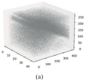
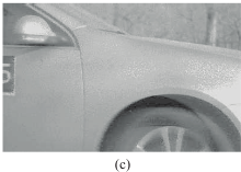
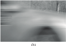
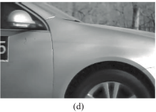
Despite these advantages, the asynchronous spike stream generated by spiking cameras is not friendly to the human visual system (Fig. 1a). It remains challenging to reconstruct dynamic scenes from asynchronous spike streams of the spiking camera. Generally, the reconstruction methods can be divided into internal statistics and deep learning methods. The internal statistics methods rebuild the scenes by estimating the firing frequency or firing interval of each pixel [Zhu et al., 2019]. Although some recent methods have incorporated the mechanism of the retina system [Zhu et al., 2020] and the short-term plasticity [Zheng et al., 2021] to enhance the estimation of the firing frequency, it is hard to balance noise and motion blur. The deep learning methods utilize end-to-end convolutional neural networks to solve the reconstruction problem and achieve better performance than internal statistics approaches [Zhao et al., 2021]. However, these methods rely on massive synthetic datasets with clean labels, while generating these datasets is still cumbersome and timeconsuming. Additionally, the spiking camera suffers distinct noises under high and low light intensity [Zhu et al., 2021], and the noise mechanisms have not been thoroughly investigated, which brings further challenges for the generation of the synthetic dataset.
In this work, we propose a novel pretext task to build a self-supervised reconstruction framework for spiking cameras, enabling us to train the network end-to-end on the realworld dataset without ground truth. Specifically, we utilize the blind-spot network commonly used in denoising tasks as our backbone and use simple internal statistics methods to construct pseudo-labels. In addition, we further excavate the potential of the blind-spot network in view of its poor scalability and insufficient information utilization, and present a mutual learning framework to improve the overall performance of the network through mutual distillation between a non-blind-spot network (NBSN) and a blind-spot network. As our NBSN is not hampered by any blind-spot constraints, state-of-the-art network architecture can be used to improve the performance. Moreover, we propose an adaptive motion inference module to obtain a better representation of the spiking data. We exploit various motion scales through temporal aggregation and inter-spike intervals [Zhu et al., 2019], which allows the network to learn from better representations.
The main contributions are summarized as follows:
- We develop a self-supervised reconstruction framework for spiking cameras by constructing a novel pretext task. To the best of our knowledge, this is the first attempt to reconstruct dynamic scenes for spiking cameras via selfsupervised learning without using a synthetic dataset.
- We propose an adaptive motion inference module to obtain a better representation for the spiking data.
- We present an effective mutual learning framework to improve the overall performance of the network. Besides, constraints of the blind-spot network can be bypassed in this approach.
- The proposed methods evidently outperform previous unsupervised methods, and achieve desirable results compared with supervised methods.
2 RelatedWork
Scene Reconstruction for Neuromorphic Vision Sensors. The event camera has shown distinctive potential in capturing high-speed and high-dynamic scenes. However, the event camera merely monitors the change of light intensity, making it challenging to record texture details in dynamic scenes [Zhao et al., 2021]. Some recent studies [Choi et al., 2020; Rebecq et al., 2019a; Rebecq et al., 2019b; Pini et al., 2018] applied deep neural networks to reconstruct images directly from events, while others [Brandli et al., 2014; Posch et al., 2008] combined traditional images and events to obtain more texture information for reconstruction. Unlike event cameras, each photosensitive unit in the spiking camera accumulates photons independently and generates a spike when the dispatch threshold is reached. The higher the light intensity, the higher the spike frequency. This property enables the spiking camera to record rich texture information. The current main reconstruction methods are based on the temporal statistic characteristic of the spiking camera [Zhu et al., 2019; Zhu et al., 2020; Zheng et al., 2021]. Zhu et al. [2019] presented two basic reconstruction methods, "texture from playback (TFP)" and "texture from inter-spike-intervals (TFI)", to rebuild the dynamic scenes from firing rate and firing interval, which requires careful choice of the window size to balance noise and motion blur. Some studies devoted to mimicking human physiological mechanisms, like retina-like visual imaging [Zhu et al., 2020] and the short-term plasticity [Zheng et al., 2021]. However, the reconstruction results of these bionic algorithms are noisy. Zhao et al. [2021] developed an end-to-end convolutional neural network and trained it on a synthetic dataset in a supervised way, which achieved state-of-the-art performance. Unfortunately, simulating large amounts of spike data is extremely challenging and expensive. Additionally, the noise mechanism of spike cameras has not been fully investigated. Thus the models trained with synthetic datasets suffer from the domain gap between synthetic and real noise.
Blind-Spot Network. Convolutional neural networks have achieved impressive performance in video denoising. However, supervised learning with large amounts of paired noisyclean images in some areas, such as CT and MRI, can be costly and even unreachable. Therefore, researchers began to focus on self-supervised denoising. Lehtinen et al. [2020] trained the network with multiple independent noisy observations per scene. Further works proposed the blind-spot network (BSN) [Lehtinen et al., 2018; Krull et al., 2019; Laine et al., 2019; Wu et al., 2020; Byun et al., 2021], which requires only one noisy observation per scene to train the network. Blind-spot means the network is designed to denoise each pixel from its surrounding spatial neighborhood without itself. Subsequent work improved the BSN by welldesigned shifted convolutions [Laine et al., 2019] and dilated convolutions [Wu et al., 2020; Byun et al., 2021]. However, these networks are carefully designed within the blind-spot constraints. Thus, some classic network modules, such as non-local attention and deformable convolution, cannot be employed directly into the network to improve performance. Huang et al. [2021] attempted to achieve self-supervised denoising without modifying the network, and can enjoy the progress of state-of-the-art network architecture design.
Mutual Learning. Knowledge distillation [Hinton et al., 2015] is a pioneering work to transfer knowledge from strong teacher networks to student networks. Recently, a variant of the knowledge distillation method called mutual learning [Zhang et al., 2018] has been proposed, breaking the "teacher-student" structure and advocating collaborative learning between a group of student networks. While most knowledge distillation methods focus on classification tasks, some methods suitable for regression tasks have been proposed [Peng et al., 2021; Wang et al., 2021; Wu et al., 2020]. In this paper, we apply the knowledge distillation for reconstruction tasks, more precisely, we present an effective mutual learning framework where a non-blind-spot network and a blind-spot network can learn from each other.
3 Methods
In this section, we first formulate the mechanism of the spiking camera, then present the whole reconstruction framework and the mutual learning strategy.
3.1 Spiking Camera
Working Mechanism
Spiking camera is composed of an H × W array of pixels, with each pixel independently accumulating the incoming light intensity L(t) persistently. When the instantaneous electric charge amount A(t) on the integrator reaches a dispatch threshold θ, a spike is fired, and then the integrator is reset to 0. The relationship between L(t) and A(t) is formulated as:
where α is the photoelectric conversion rate.
Although spikes can fire at arbitrary time tk given A(tk) = 0, it can only be read out by checking the spike flag at discrete times due to the limitations of circuit technology. Specially, the camera checks the spike flag periodically with a fixed interval T = 25 µs. A spike will be read out S(n) = 1 (n = 1, 2, . . .) if the spike flag has been set up at the time t, with (n - 1)T < t ⩽ nT . Otherwise it reads out S(n) = 0. Considering that all the pixels on the sensor continuously accumulate the incoming light and fire spikes independently, the spiking camera would produce a continuous binary spike stream S ∈ {0, 1}H×W×N during the period [0, NT ].
Basic Reconstruction Methods
The goal of scene reconstruction of the spiking camera is to restore the intensity images {In|In ∈ [0, 255]H×W , n = 1, 2, . . .N} from the output spike stream S ∈ {0, 1}H×W×N . The basic reconstruction methods are "texture from play-back (TFP)" and "texture from inter-spike-intervals (TFI)" [Zhu et al., 2019], utilizing that the photosensitive units of spiking camera receive different scene radiance will trigger spikes with different frequencies.
The TFP method obtains the pixel value by calculating the number of spikes in a time window, which is formulated as:
where I TFP n refers to the pixel value at moment n, w is the size of time window, Nw is the total number of spikes collected in the time window, and the C refers to the maximum dynamic range of the reconstruction.
The TFI method assumes that the scene radiance L(t) is a constant L in a short period. According to Eq. 1, the spike generation can be simplified as L∆t ≥ θ, where ∆t is the inter-spike interval (ISI) obtained by calculating the time between two neighboring spikes. Thus, the pixel value can be estimated with two spikes:
where ∆tn represents the ISI corresponding to moment n.
3.2 Self-Supervised Reconstruction Network Overview Architecture
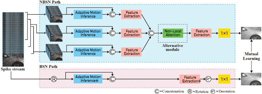
In this section, we propose the self-supervised reconstruction framework. The overall network structure is illustrated in Fig. 2, which takes a consecutive spike stream S ∈ {0, 1}H×W×N as input. The network consists of two reconstruction paths, one is a blind-spot network (BSN), and the other is a non-blind-spot network (NBSN), i.e. an unprocessed conventional convolutional neural network. The NBSN path process the input stream in a two-stage manner commonly used in video processing [Sheth et al., 2021; Tassano et al., 2020]. In the first stage, the input spike stream is split into three overlapping sub-stream {St-k, St, St+k}, where St denotes the sub-stream around time t and k denotes the overlap size. Next, each sub-stream goes through the Adaptive Motion Inference Module, producing coarse estimation features {Ft-k, Ft, Ft+k} under attention weighting. Then each concatenation of the estimation features and the sub-stream is sent to the Feature Extraction Module (a modified share-weight U-Net) to extract further features { ˆ Ft-k, ˆ Ft, ˆ Ft+k}. In the second stage, a Non-Local Attention Module is applied to fuse these features to strengthen feature representations. Finally, the fused features are sent to another modified U-Net followed by 1 × 1 convolutions to reconstruct the final clean image ˆ It. The working flow of the BSN path follows a one-stage manner. Specifically, the input spike stream is fed into the Adaptive Motion Inference Module directly, then a modified U-Net followed by 1 × 1 convolutions is applied to the concatenated output to produce the final reconstruction result. The two paths are jointly trained using mutual learning paradigm.
Adaptive Motion Inference Module (AMIM)
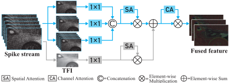
A continuous spike stream contains multiple spike frames, which provide rich information to reconstruct the highquality image. However, because of the complexity of the motion scene, extracting appropriate features remains challenging. Inspired by the fact that TFI and TFP methods are suitable for dealing with moving and stationary scenes respectively[Zhu et al., 2019], we propose an attention-based AMIM to extract more valuable features from these two basic reconstruction methods (Fig. 3). First, in the stationary branch, three sets of masks and 1×1 convolutions are used to perform multi-scale temporal aggregation imitating the process of TFP:
where M 1 i is the mask of the i-th scale, ft 1i denotes the corresponding 1 × 1 convolution and ◦ denotes element-wise multiplication. Then a spatial attention block M 1 s (·) is used on the concatenated output to find the stationary area.
where [, ] denotes feature concatenation.
Second, in the motion path, the TFI reconstruct I TFI t is fed into a 1 × 1 convolution f 2 t (·) and spatial attention block M 2 s (·) to find the motion area.
Finally, a channel attention block Mc is introduced to obtain the final fused features ˆ Ft:
where ⊕ denotes the element-wise sum.
Pretext Task Using Blind-Spot Network
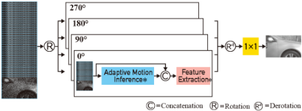
We build the BSN framework using the blind-spot strategy proposed in [Laine et al., 2019] to estimate each output pixel from a spatio-temporal neighborhood without the pixel itself. The training of the BSN does not require noisy-clean image pairs. Instead, it utilizes the noisy image itself as both input and supervision signals.The blind-spot constraint will prevent the network from learning identity mapping to noisy images, but produce clean results. These motivate us to use BSN as our backbone to achieve self-supervision and clean output. A natural idea is to use noisy TFI (or TFP) as both input and supervision signal, while in order to fully mine the rich temporal information of spike stream, we take the spike stream as the input.
In our BSN framework (Fig. 4), the rotated versions of the input spike stream are concatenated together in the batch dimension. Then we pass the input through the shifted-conv based BSN, leading to an output with four times the number of batch-size. After that, the output reverts into four parts in the batch dimension and concatenated together in the channel dimension, and finally passes through 1 × 1 convolutions to produce the estimated reconstruction image ˆ I bsn t .
We use the self-supervised denoising task as a pretext task to train the network. We hope that the BSN can remove the Spike frame TFP 23.49 dB TFI 23.21 dB TVS 11.36 dB
GT
Spike frame TFP 21.16 dB TFI 24.47 dB TVS 12.29 dB
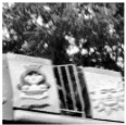
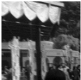
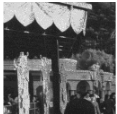
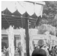
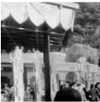
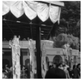
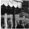
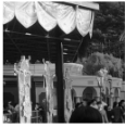
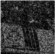
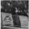
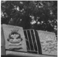
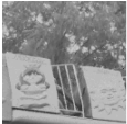
Figure 5: Evaluation of different methods on synthetic dataset.
noise and improve the details of the latent image in the spike stream, so as to output high-quality noiseless reconstruction images. In order to train the network reasonably and effectively, it is necessary to find appropriate pseudo-labels for self-supervision. As discussed in Sec. 3.1, we can utilize simple internal statistics results, such as TFI or TFP as the noisy label to train the network. We refer to the pseudo-label as Ipseudo, and the reconstruction loss function can be formulated as:
The use of the BSN ensures that the network trained with TFI (or TFP) as pseudo-labels will not learn to reconstruct labels themselves, but learn their latent clean representations.
Mutual Learning Strategy
The BSN framework faces the following problems:
- The blind-spot network relies heavily on specific convolution kernel design, which leads to poor network scalability. Thus the state-of-the-art modules in supervised learning can not be applied to the network directly.
- The nature of the blind-spot makes it impossible for each pixel of the output to obtain information from the corresponding position of the input, which reduces the utilization of information by the network compared to normal CNNs.
- The rotation operation makes the input batch-size quadruple the original size. Besides, due to the overlapped receptive fields of different rotation versions, the input pixels are processed twice, resulting in redundant calculation and a high inference cost.
Among them, the first two are common problems of most blind-spot networks [Krull et al., 2019; Laine et al., 2019; Wu et al., 2020; Byun et al., 2021], and the third is unique to the network we use in Sec. 3.2
To address these issues, we propose a mutual learning paradigm between the BSN and the NBSN. As the NBSN is a normal convolution network, we can add modules popular in supervised learning without limitations. In this paper we use a separated non-local attention module (green box in Fig. 2) [Huang et al., 2019; Fu et al., 2019; Wang et al.,
2018]. Specifically, criss-cross spatial attention [Huang et al., 2019], channel attention, and temporal attention are applied to the concatenated feature of the outputs of first stage separately to exploit the long-term temporal correlation.
In our mutual learning framework, both BSN and NBSN can be regarded as "student network", while learning collaboratively and implicitly transfer useful knowledge to each other. The BSN provides the NBSN with "clean" features learned by the blind-spot strategy, meanwhile, the NBSN, as a "stronger student" with more temporal correlation information and powerful modules, promotes the BSN with more refined information. For the classification tasks, KL-divergence is used as mutual learning loss to utilize soft labels for knowledge transfer [Zhang et al., 2018]. For the regression task, we define the mutual learning loss function as
and the total loss function can be formulated as
where λ is a weighting parameter. After training, we only use the NBSN path to produce reconstruction images, thus the high computational cost of the BSN path can be avoided.
4 Experiments
We evaluate the performance of our method on both synthetic and real-world datasets.
4.1 Evaluation on Synthetic Dataset
Synthetic Dataset
For quantitative evaluation, we use the synthetic dataset with ground truth to train our network, which is obtained from SpkImgNet [Zhao et al., 2021]. This synthetic dataset is generated by converting videos from REDS [Nah et al., 2019] to spike stream, with frames in the videos as the ground truth. The training set consists of 800 spike stream-ground truth pairs with a spatial resolution of 400 × 250, and the testing set consists of 40 spike stream-ground truth pairs of the same size. We compare our method with previous representative reconstruction works, including TFI and TFP [Zhu et al., 2019], TVS [Zhu et al., 2020], STP [Zheng et al., 2021] and Spk2ImgNet [Zhao et al., 2021].
(a) Spike frame
(b) TFI
(c) TFP
(d) TVS
(e) STP
| Methods | Supervised | Unsurpervised | ||||
|---|---|---|---|---|---|---|
| Spk2ImgNet | TFI | TFP | TVS | STP | Ours | |
| PSNR | 38.44 | 24.94 | 22.37 | 23.15 | 22.37 | 34.26 |
| SSIM | 0.9767 | 0.7150 | 0.5801 | 0.7452 | 0.7300 | 0.9718 |
| Scene | Sample rate | Resolution | Description |
|---|---|---|---|
| Car | 20,000 Hz | 400 × 250 | 100 km/h |
| Doll | 20,000 Hz | 400 × 250 | Free fall |
| Fan | 40,000 Hz | 400 × 250 | 2600 rpm |
| Train | 20,000 Hz | 400 × 250 | 350 km/h |
Table 2: Details of real-world dataset.
Qualitative and Quantitative Evaluation
Here PSNR and SSIM are used to compare our method with previous methods quantitatively. As illustrated in Tab. 1, our method outperforms the previous unsupervised methods evidently. The performance of our method is slighter lower than Spk2ImgNet. However, as a supervised method, the training of Spk2ImgNet depends on a large synthetic dataset with ground truth, and generating the dataset through a spike simulator is a cumbersome and time-consuming task. In contrast, our self-supervision method can be trained directly on the real world dataset, which can be easily obtained by the spiking camera. The reconstruction results of compared methods are illustrated in Fig. 5.
4.2 Evaluation on Real World Dataset
We also compare our methods with the state-of-the-art methods on real-world dataset captured by the spiking camera with a sampling rate of 40,000 Hz. This dataset consists of four different sequences, including high-speed scenes with the object's motion and high-speed scenes with the camera's egomotion, such as a rotating fan with 2600 rpm (revolutions per minute) and high-speed trains in 350 km/h, etc. Please refer to Table. 2 for more information.
| Methods | Supervised | Unsurpervised | ||||
|---|---|---|---|---|---|---|
| Spk2ImgNet | TFP | TFI | TVS | STP | Ours | |
| Car | 4.0028 | 7.6423 | 13.0197 | 9.3054 | 5.5144 | 3.7595 |
| Doll | 3.9737 | 8.2026 | 7.9594 | 7.4768 | 7.3340 | 5.3591 |
| Fan | 3.7233 | 7.2340 | 11.9794 | 6.2319 | 4.6580 | 4.5007 |
| Train | 3.7140 | 6.4892 | 10.6230 | 6.7824 | 5.1873 | 3.6053 |
| Average | 3.8532 | 7.3920 | 10.8954 | 7.4491 | 5.6734 | 4.3061 |
| Methods | PSNR | SSIM |
|---|---|---|
| BSN | 32.96 | 0.9604 |
| BSN+AMIM | 33.23 | 0.9635 |
| BSN+AMIM+LTC | 28.25 | 0.9102 |
| BSN+AMIM+LTC+NLA | 25.45 | 0.8106 |
As shown in Fig. 6, our method achieves better performance than the unsupervised methods. Specifically, the TFP method suffers from severe motion blur under larger window size, and appears to be noisy under smaller window sizes. The TFI, TVS and the STP-based method can restore the motion area effectively, while the appearance of noise can not be ignored. Furthermore, our method has achieved almost the same qualitative performance as the supervised method, with clean textures and rich details. Similar to Spk2ImgNet, we use a no-reference image quality assessment metric named NIQE to evaluate the performance of different scenes on the real-world dataset. As shown in Tab. 3, our method outperforms previous unsupervised reconstruction methods and achieves comparable performance to the supervised method.
(f) Spike2ImgNet
(g) Ours TFP (w=15)
TFP (w=19)
| Methods | PSNR | SSIM |
|---|---|---|
| BSN & NBSN | 33.83 | 0.9680 |
| BSN & NBSN+LTC | 34.01 | 0.9701 |
| BSN&NBSN+LTC+NLA | 34.26 | 0.9718 |
Table 5: Ablation study for different network configurations of the two student network in mutual learning.
4.3 Ablation Study
Reconstruction without Mutual Learning
In this section, we explore the effect of the proposed modules and demonstrate the limitations of a single BSN through experiments on the synthetic dataset. The experiments are conducted in a single BSN. Specifically, the mutual learning strategy is not used. As shown in Table 4, a single BSN with the proposed AMIM module performs best, indicating that the proposed AMIM can provide a better representation for spike stream through adaptive motion inference. Besides, we notice that BSN with long-term temporal correlation (LTC) does not show the expected performance, which we attribute to the lack of explicit temporal fusion.
Moreover, BSN with LTC and a non-local attention (NLA) module performs poorly. It is because the non-local nature of this module breaks the blind-spot constraint that an output pixel can only obtain information from its surrounding spatial neighborhood without itself. With these experiments, we have demonstrated the poor scalability of a single BSN without mutual learning. As BSN with LTC and NLA breaks the blind-spot constraint of the denoising pretext task, these results can also be regarded as ablation for the pretext task.
Reconstruction with Mutual Learning
We further evaluate the effect of different network configurations of the two student networks in mutual learning. Note that the AMIMmodule is employed in all networks listed in the Tab. 5 in order to reduce unnecessary experiments. As shown in Tab. 5, the combination of an NBSN with LTC followed by a NLA module and a BSN with only short-term temporal correlation performs best, which outperforms the best network in Tab. 4 by around 1 dB. It indicates that our mutual learning strategy can transfer valuable knowledge to each other to improve performance.
| Pseudo-Labels | PSNR | SSIM |
| TFI | 33.09 | 0.9605 |
| TFP(w = 7) | 34.19 | 0.9713 |
| TFP(w = 11) | 33.94 | 0.9695 |
| TFP(w = 15) | 33.41 | 0.9657 |
| TFP(w = 19) | 32.81 | 0.9599 |
We also notice that even the simple combination of a BSN and NBSN with the same structure can achieve better performance than a single BSN, and the performance will improve with the addition of more modules in the NBSN, which implies that the poor scalability of BSN can also be bypassed through our mutual learning strategy.
Effect of Different Pseudo-Labels
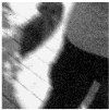
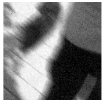
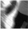
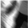
Table. 6 shows the performance trained with different pseudolabels on the proposed network. Note that the performance decreases as windows grow, as larger windows may introduce more motion blur, which can be seen in Fig. 7.
4.4 Implementation Details
The parameter λ of the loss function is set to 0.01, and the input spike stream is cropped into 40 × 40 patches with a batch size of 4. Besides, we set the short-term temporal window size and long-term temporal window size to 41 and 27, respectively, and remove all additive terms from the convolutional layer as in [Sheth et al., 2021] for better generalization. Moreover, we use Adam optimizer with the default setting to optimize our network, and train the network with TFP (w = 7) as pseudo labels on Nvidia RTX 2080 GPU for 100k iterations. The BSN path is first trained for 15k iterations before mutual learning.
5 Conclusions
In this paper, we present an end-to-end self-supervised mutual learning framework to address the reconstruction problem of the spiking camera. We adopt the blind-spot network into the reconstruction problem and construct a proper selfsupervised pseudo-label by utilizing the two basic reconstruction methods, TFI and TFP. To overcome the limitations of the blind-spot network, we propose a mutual learning strategy for knowledge transfer between a non-blind-spot network and a blind-spot network. Experiments on both synthetic and real-world datasets have demonstrated that the proposed framework can restore pleasant and high-quality images from spike streams and achieve comparable results as the supervised method. To the best of our knowledge, this is the first attempt to restore dynamic scenes from the spiking camera in a self-supervised manner without using any synthetic dataset.
Acknowledgments
This work was supported by the National Key Research and Development Program of China (Grant No.2021ZD0200300) and the National Natural Science Foundation of China (Grant No.62176003 and No.62088102).
@inproceedings{ijcai2022p396,
  title     = {Self-Supervised Mutual Learning for Dynamic Scene Reconstruction of Spiking Camera},
  author    = {Chen, Shiyan and Duan, Chaoteng and Yu, Zhaofei and Xiong, Ruiqin and Huang, Tiejun},
  booktitle = {Proceedings of the Thirty-First International Joint Conference on
               Artificial Intelligence, {IJCAI-22}},
  publisher = {International Joint Conferences on Artificial Intelligence Organization},
  editor    = {Luc De Raedt},
  pages     = {2859--2866},
  year      = {2022},
  month     = {7},
  note      = {Main Track},
  doi       = {10.24963/ijcai.2022/396},
  url       = {https://doi.org/10.24963/ijcai.2022/396},
}
TY - CPAPER TI - Self-Supervised Mutual Learning for Dynamic Scene Reconstruction of Spiking Camera AU - Chen, Shiyan AU - Duan, Chaoteng AU - Yu, Zhaofei AU - Xiong, Ruiqin AU - Huang, Tiejun T2 - Proceedings of the Thirty-First International Joint Conference on Artificial Intelligence, IJCAI-22 PB - International Joint Conferences on Artificial Intelligence Organization PY - 2022 SP - 2859 EP - 2866 DO - 10.24963/ijcai.2022/396 UR - https://doi.org/10.24963/ijcai.2022/396 ER -Copied
Machine-readable versions of this paper, for tools and AI agents:





