
Multi-Vector Embedding on Networks with Taxonomies
Proceedings of the Thirty-First International Joint Conference on Artificial Intelligence. Main Track. Pages 2944-2950.
https://doi.org/10.24963/ijcai.2022/408
Keywords
- Data Mining: Mining Heterogenous Data
- Machine Learning: Multi-label
- Multidisciplinary Topics and Applications: Bioinformatics
- Machine Learning: Representation learning
- Data Mining: Networks
Abstract
A network can effectively depict close relationships among its nodes, with labels in a taxonomy describing the nodes' rich attributes. Network embedding aims at learning a representation vector for each node and label to preserve their proximity, while most existing methods suffer from serious underfitting when dealing with datasets with dense node-label links. For instance, a node could have dozens of labels describing its diverse properties, causing the single node vector overloaded and hard to fit all the labels. We propose HIerarchical Multi-vector Embedding (HIME), which solves the underfitting problem by adaptively learning multiple 'branch vectors' for each node to dynamically fit separate sets of labels in a hierarchy-aware embedding space. Moreover, a 'root vector' is learned for each node based on its branch vectors to better predict the sparse but valuable node-node links with the knowledge of its labels. Experiments reveal HIME’s comprehensive advantages over existing methods on tasks such as proximity search, link prediction and hierarchical classification.
- [Ashburner et al., 2000] Michael Ashburner, Catherine A Ball, Judith A Blake, David Botstein, Heather Butler, J Michael Cherry, Allan P Davis, Kara Dolinski, Selina S Dwight, Janan T Eppig, et al. Gene ontology: tool for the unification of biology. Nature genetics, 25(1):25-29, 2000.
- [Davis et al., 2020] Allan Peter Davis, Cynthia J Grondin, Robin J Johnson, Daniela Sciaky, Jolene Wiegers, Thomas C Wiegers, and Carolyn J Mattingly. Compara- tive Toxicogenomics Database (CTD): update 2021. Nu- cleic Acids Research, 49(D1):D1138-D1143, 10 2020.
- [Epasto and Perozzi, 2019] Alessandro Epasto and Bryan Perozzi. Is a single embedding enough? learning node rep- resentations that capture multiple social contexts. In The World Wide Web Conference, page 394-404. Association for Computing Machinery, 2019.
- [Grover and Leskovec, 2016] Aditya Grover and Jure Leskovec. node2vec: Scalable feature learning for networks. In Proceedings of the 22nd ACM SIGKDD international conference on Knowledge discovery and data mining, pages 855-864, 2016.
- [Hamilton et al., 2017] Will Hamilton, Zhitao Ying, and Jure Leskovec. Inductive representation learning on large graphs. In Advances in Neural Information Processing Systems, volume 30, 2017.
- [Hao et al., 2019] Junheng Hao, Muhao Chen, Wenchao Yu, Yizhou Sun, and Wei Wang. Universal representation learning of knowledge bases by jointly embedding in- stances and ontological concepts. In Proceedings of the 25th ACM SIGKDD International Conference on Knowl- edge Discovery and Data Mining, page 1709-1719, 2019.
- [Huntley et al., 2015] Rachael P Huntley, Tony Sawford, Prudence Mutowo-Meullenet, Aleksandra Shypitsyna, Carlos Bonilla, Maria J Martin, and Claire O'Donovan. The goa database: gene ontology annotation updates for 2015. Nucleic acids research, 43(D1):D1057-D1063, 2015.
- [Liu et al., 2015] Zhi-Ping Liu, Canglin Wu, Hongyu Miao, and Hulin Wu. RegNetwork: an integrated database of transcriptional and post-transcriptional regulatory net- works in human and mouse. Database, 2015, 09 2015. bav095.
- [Liu et al., 2019] Ninghao Liu, Qiaoyu Tan, Yuening Li, Hongxia Yang, Jingren Zhou, and Xia Hu. Is a single vector enough? exploring node polysemy for network em- bedding. In Proceedings of the 25th ACM SIGKDD Inter- national Conference on Knowledge Discovery and Data Mining, page 932-940, 2019.
- [Nickel and Kiela, 2017] Maximillian Nickel and Douwe Kiela. Poincaré embeddings for learning hierarchical rep- resentations. In Advances in Neural Information Process- ing Systems, volume 30, 2017.
- [Nickel and Kiela, 2018] Maximilian Nickel and Douwe Kiela. Learning continuous hierarchies in the lorentz model of hyperbolic geometry. In Proceedings of the 35th International Conference on Machine Learning, vol- ume 80, pages 3776-3785, 2018.
- [Park et al., 2020] Chanyoung Park, Carl Yang, Qi Zhu, Donghyun Kim, Hwanjo Yu, and Jiawei Han. Unsuper- vised differentiable multi-aspect network embedding. In Proceedings of the 26th ACM SIGKDD International Con- ference on Knowledge Discovery and Data Mining, pages 1435-1445, 2020.
- [Petri et al., 2014] Victoria Petri, Pushkala Jayaraman, Marek Tutaj, G. Thomas Hayman, Jennifer R. Smith, Jeff De Pons, Stanley JF Laulederkind, Timothy F. Lowry, Ra- jni Nigam, Shur-Jen Wang, Mary Shimoyama, Melinda R. Dwinell, Diane H. Munzenmaier, Elizabeth A. Worthey, and Howard J. Jacob. The pathway ontology -updates and applications. Journal of Biomedical Semantics, 5(1):7, Feb 2014.
- [Ren et al., 2016] Xiang Ren, Wenqi He, Meng Qu, Lifu Huang, Heng Ji, and Jiawei Han. Afet: Automatic fine- grained entity typing by hierarchical partial-label embed- ding. In Proceedings of the 2016 conference on empiri- cal methods in natural language processing, pages 1369- 1378, 2016.
- [Szklarczyk et al., 2021] Damian Szklarczyk, Annika L Gable, Katerina C Nastou, David Lyon, Rebecca Kirsch, Sampo Pyysalo, Nadezhda T Doncheva, Marc Legeay, Tao Fang, Peer Bork, et al. The string database in 2021: cus- tomizable protein-protein networks, and functional char- acterization of user-uploaded gene/measurement sets. Nu- cleic acids research, 49(D1):D605-D612, 2021.
- [Tang et al., 2015] Jian Tang, Meng Qu, and Qiaozhu Mei. Pte: Predictive text embedding through large-scale hetero- geneous text networks. In Proceedings of the 21th ACM SIGKDD international conference on knowledge discov- ery and data mining, pages 1165-1174, 2015.
- [Wang et al., 2018] Hongwei Wang, Jia Wang, Jialin Wang, Miao Zhao, Weinan Zhang, Fuzheng Zhang, Xing Xie, and Minyi Guo. Graphgan: Graph representation learning with generative adversarial nets. In Proceedings of the AAAI conference on artificial intelligence, volume 32, 2018.
- [Wang et al., 2019] Junshan Wang, Zhicong Lu, Guojia Song, Yue Fan, Lun Du, and Wei Lin. Tag2vec: Learning tag representations in tag networks. In The World Wide Web Conference, page 3314-3320, 2019.
- [Yang et al., 2020] Carl Yang, Jieyu Zhang, and Jiawei Han. Co-embedding network nodes and hierarchical labels with taxonomy based generative adversarial networks. In 2020 IEEE International Conference on Data Mining (ICDM), pages 721-730. IEEE, 2020.
References were extracted automatically from the PDF and may contain errors.
Full text extracted automatically from the PDF; figures, tables and equations may differ. The PDF is the version of record.
1 Introduction
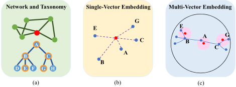
A network is able to depict the proximity among nodes. Extra node properties are described by labels organized as a taxonomy, which is often presented as a directed acyclic graph (DAG). For instance, in a Protein-Protein Interaction (PPI) network with Gene Ontology (GO) being the taxonomy, network edges reveal interactions among proteins, while different hierarchical GO terms of a protein tell its diverse biological properties. Generally, a node can have multiple label paths in the taxonomy, as shown in figure 1 (a).
Traditional heterogeneous network embedding methods serve as an option for co-embedding the network and the taxonomy. They learn a representation vector for each node and label, so that the proximity is preserved by the distances among the vectors. However, on datasets with dense nodelabel relationships, the single representation vector of a node could be overloaded and hard to fit the node's different labels, which causes the underfitting problem [Yang et al., 2020]. As illustrated in figure 1 (b), in order to minimize the overall distance to its labels, the node vector is embedded near the center of its five labels without being close to any of them. This underfitting problem seriously decreases the quality of the representation vectors, causing them containing vague or even misleading information.
∗Corresponding author: Xiuli Ma.
To solve the underfitting problem, one way is to optimize the positions of the labels so as to minimize the probability of underfitting, which can be achieved by the Poincar´e ball model [Nickel and Kiela, 2017]. A Poincar´e ball is a hyperbolic space with constant negative curvature of -1, and can be viewed as a continuous version of trees. It naturally caters to the taxonomy, with high-level labels embedded near the origin while low-level ones near the ball surface, and labels in a label-path embedded in the same direction. Therefore, a node vector is less likely to underfit labels belonging to a single label path. But using the Poincar´e ball alone does not necessarily tackle the underfitting problem, since a node can have multiple label paths embedded away from each other.
Based on the Poincar´e ball, an effective way to solve the underfitting problem is to 'divide and conquer'. Specifically, we allow multiple 'branch vectors' for each node to fit different sets of its labels. A branch vector can reflect a group of closely related low-level characteristics, or indicate the general concepts that the node belongs to. Therefore, multivector embedding provides a more accurate and hierarchical representation as shown in figure 1 (c). The branch vector number is adaptive to the node's label distribution. Besides, the Least Recently Used (LRU) policy is employed to balance the loads among the branch vectors of the node.
The branch vectors can then be utilized in preserving sparse but valuable node-node relationships. In a gene regulatory network for instance, it is expensive and intractable to biologically examine all the regulations among up to 27000 human genes, making the label information crucial for predicting unseen regulations. Given a node with its label information learned by its branch vectors, we use a single 'root vector' aggregating these information to better preserve existing links and predict the potential ones.
We conclude our method as HIerarchical Multi-vector Embedding (HIME), which learns a representation vector for each label and multiple branch vectors for each node to fit its different label clusters. A single root vector is then learned for each node based on its branch vectors to preserve node-node proximity. Our work makes the following contributions: (1) We propose multi-vector embedding to solve the underfitting problem. (2) The LRU policy is applied to balance the loads among the branch vectors. (3) The root vector aggregated from the branch vectors better preserves the node proximity. (4) We conduct extensive experiments to show HIME's comprehensive advantages over existing methods.
2 RelatedWork
Network embedding aims at learning representation vectors for network nodes to preserve the node proximity. The methodologies of network embedding can be mainly categorized into matrix factorization, Skip-Gram with walk patterns [Grover and Leskovec, 2016; Tang et al., 2015] and neural networks [Wang et al., 2018]. These classic methods laid the foundation for later variants such as taxonomy-related embedding and multi-aspect embedding.
2.1 Taxonomy-Related Embedding
Most taxonomy-related embedding methods co-embed network nodes and taxonomy labels. Unlike the entity typing task [Ren et al., 2016] in natural language processing that focuses on preserving node-label relationships, taxonomyrelated network embedding should take both node-node and node-label relationships into account.
Poincar´e [Nickel and Kiela, 2017] and Lorentz [Nickel and Kiela, 2018] both embed WordNet into a hyperbolic space so as to maintain the hypernym relationships. The hyperbolic space is later applied by Tag2Vec [Wang et al., 2019] that co-embeds the network and the taxonomy by Skip-Gram with meta-paths. The three methods ensure the universality of the embedding vectors by using a single hyperbolic space, but they suffer from the underfitting problem. JOIE [Hao et al., 2019] embeds nodes and labels into two separate spaces connected by a non-linear affine transformation. TaxoGAN [Yang et al., 2020] spares an individual embedding space for every label where its nodes and its child labels are embedded by adversarial training, while its drawback is also obvious since the representation vectors only function locally in diverse spaces.
In general, these taxonomy-related methods are blocked by the trade-off between the universality and the accurateness of the representation vectors. By contrast, HIME generates a precise embedding in a single Poincar´e ball.
2.2 Multi-Aspect Embedding
Several recent works have revealed the necessity of learning multiple vectors to capture different aspects of the node. For instance, PolyDW [Liu et al., 2019] represents each facet of an item using a single vector, and Splitter [Epasto and Perozzi, 2019] allows multiple node embedding vectors to encode different communities. The drawback of them is that the aspects of the node need to be determined in advance and are fixed during the learning process, while Asp2Vec [Park et al., 2020] employs random walks to dynamically assign aspects to each node according to its local context.
Though multiple vectors are learned for each node, given a specific aspect, these methods are in essence single-vector embedding since each node has only a single vector in an aspect. By contrast, the computation of the distance between a node and a label in HIME involves all the node's branch vectors and the label vector.
3 Problem Statement
HIME takes the following data as inputs:
- a network N = {V, E}, where V = {v1, v2, ..., vn} is the set of nodes, and E = {ei,j}ni,j is the set of edges.
- a taxonomy T = {L, U}, where L = {l1, l2, ..., lm} is the set of labels, and U = {(li, lj) | lj ∈ Pa(li)} is the set of parent-child edges, where Pa(li) is the set of li's parents in the DAG.
- The label assignment A = A1 ∪ A2 ∪ ... ∪ An, where Ai is the set of node-label links of node vi. Once a label appears in Ai, its ancestors will also appear in Ai.
HIME learns a vector for each label and multiple vectors for each node. A node has several 'branch vectors' to fit its labels and a single 'root vector' to preserve its node-node proximity. Formally, given branch limit K, HIME learns:
- a set of label vectors Q = {q1, q2, ..., qm}, with qi referring to the representation vector of label li.
- a set of branch vectors B = B1 ∪ B2 ∪ ... ∪ Bn, where Bi = {bi,1, bi,2, ..., bi,ki } is the set of ki branch vectors of node vi. ki ≤K.
- a set of root vectors R = {r1, r2, ..., rn}, with ri being the root vector of node vi.
4 Method
4.1 The Poincar´e Ball
Let ‖·‖ denotes the Euclidean L2 norm. A Poincar´e ball with dimension d and radius 1 can be defined as the Riemannian manifold: P d,1 := {x ∈ Rd | ‖x‖2 < 1}, gx = λ2xId, where gx is the Riemannian metric tensor, λx = 2/(1 - ‖x‖2 ) and Id is the identity matrix. The distance between two points x, y ∈ P d,1 can be computed as:
With ‖x-y‖ fixed, the distance d(x, y) grows rapidly to infinity when ‖x‖ approaching the open boundary 1, similar to a tree that expands exponentially with the increase of the tree depth. [Nickel and Kiela, 2017] first used the Poincar´e ball to embed hierarchical data.
4.2 Multi-Vector Embedding
The multi-vector embedding (MVE) procedure in HIME is to learn a representation vector for each label and an adaptive number of branch vectors for each node to fit its separate label sets. Inspired by the K-means algorithm, which clusters data points by assigning them to their closest centroids, we view the branch vectors as the centroids and the labels as the points to be clustered. The main difference is that the points are fixed in the clustering task, while the label vectors can be dynamically optimized in MVE.
Here we discuss the adaptiveness of MVE by examining the K-means algorithm. In the K-means, though the number K of the centroids is predetermined, the final number of clusters could be less than K if no data points are assigned to some centroids. It will happen when a poor centroid initialization is made or the point number has the same or close order of magnitude to K. The later situation indicates that the number of clusters can be adaptive to the distribution of a relatively small number of points, which is often the case in preserving about a dozen of labels by using several branch vectors. We present the details of MVE as follows.
The Mechanism of Multi-Vector Embedding
We first allocate K branch vectors bi,1, bi,2, ..., bi,K for each node vi, and initialize all the branch vectors and the label vectors close to the origin of the Poincar´e ball. We define the node-label distance between node vi and label lj as the shortest Poincar´e distance from all the branch vectors {bi,1, bi,2, ..., bi,K} to the label vector qj:
Parallel computation of this node-label distance can be easily implemented for a batch of node-label pairs. We then optimize the branch vectors and the label vectors by the following objective function with negative sampling:
where Aneg contains negatively sampled node-label links. It should be pointed out that the positive set A can also include potential node-label links by performing random walks on meta-path 'Node-Node-Label' based on the dataset-specific assumption that connected nodes will have similar labels.
By maximizing Onl, the negative samples serve as a strong force to push the branch vectors and the label vectors away from each other and the origin. By contrast, the positive samples has the clustering effect. Given a node-label pair (vi, lj), suppose bi,1 is the branch vector closest to qj among all vi's branch vectors, and in this way, D(vi, lj) = d(bi,1, qj). During the back propagation process, only the gradients of bi,1 and qj are updated by (vi, lj). Therefore, if (vi, lj) is a positive sample, D(vi, lj) will be decreased, which means that
Algorithm 1 The LRU policy.
- 1: for i in n nodes do 2: get hitmin, idmin =min(Hi,1,Hi,2, ...,Hi,K) 3: get hitmax, idmax =max(Hi,1,Hi,2, ...,Hi,K) 4: if hitmin == 0 then 5: sample ϵ from normal distribution N(0, 10-6 ) 6: bi,idmin ← expbi,idmax (ϵ) 7: end if 8: end for
both bi,1 and qj will be updated closer. It can be interpreted in a way that given a node, a label is always assigned to the closest branch vector of the node, while a branch vector fits a cluster of labels, with all the vectors optimized dynamically.
Tracing the Active Branch Vectors
We call a node's branch vector 'active' if at least one of the node's labels is assigned to it, otherwise we call it 'inactive'. The active branch vectors are those we want in the end. We maintain a hit matrix Hn×K , where Hi,a records the number of labels that bi,a fits at the end of every epoch. Therefore, ∑Ka=1 Hi,a = ‖Ai‖, where Ai is the label set of vi. H is set to 0 at the beginning of every epoch, and it can be simply maintained by the procedure computing the node-label distance. Given a positive pair (vi, lj), the procedure remembers the index id of the branch vector closest to qj when computing the node-label distance, and plus Hi,id by 1 to record a hit. At the end of the MVE, we pick the active branch vectors according to their non-zero hit value in the last epoch.
The LRU Load Balancing Policy
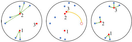
Since all the vectors are dynamically updated, sometimes unbalanced loads are shared among a node's branch vectors. In figure 2, the hit values of the three red branch vectors are 2, 5 and 0 at the beginning. MVE almost degenerates into single vector embedding since the busiest branch vector fits a majority of labels. We use a least-recently-used (LRU) policy to balance the loads among the branch vectors.
The main idea is to split the most active vector into two vectors so that each is assigned a smaller set of labels. The two vectors are then optimized in the following epochs to fit its label clusters. With H providing the hit values, the 'splitting' can be achieved by replacing an inactive branch vector (LRU vector) close to the most active branch vector with a small randommargin between them, so as to share the burden of the most active vector, as shown in figure 2. Algorithm 1 describes the LRU policy, where expx(y) updates x with a step y in the Poincar´e ball (see appendix 1 ).
4.3 Refining the Label Hierarchy
MVE can roughly generate a hierarchical embedding of the taxonomy in a way that a high-level label having more nodes will be placed near the origin so as to minimize the overall Poincar´e distance to its nodes, while low level labels with few nodes will be embedded near the boundary due to the effect of negative sampling. But with the ground-truth information given by T , a more accurate embedding of the label hierarchy could be further achieved.
One thought is to simply use the Poincar´e distance to reflect the relationships between two labels. However, though the Poincar´e distance can reflect the proximity, it fails to reflect the partial order among the labels since the distance is symmetric for the two input vectors. Therefore, an asymmetric score function is required for directed parent-child edges.
Given two labels li and lj, we call li 'is a' lj if li ≺ lj, meaning that there is a directed DAG path from lj to li. We define the asymmetric score function of relation 'is a' as:
where α is a positive hyper-parameter set to 1. If qi and qj are close in the Poincar´e ball and qj is closer to the origin than qi, then a high score Sis a(li, lj) will indicate the probability of li ≺ lj, particularly, li being the child of lj. This score function is first introduced by [Nickel and Kiela, 2017] in the experimental evaluation, and here we apply it in the refinement of the label vectors:
Where U is the parent-child edge set and Uneg is the set of negative edges sampled from {(li, lj)|li ̸≺ lj}. By maximizing Oll, the label vectors will be refined according to both the proximity and the partial order. The refinement of the label vectors is performed together with MVE.
4.4 Learning the Root Vector
A single root vector is learned for each node based on its active branch vectors to preserve the network proximity. This procedure is after MVE, since the active branch vectors of a node are not determined until the end of MVE.
Specifically, we use the hyperbolic aggregation over the branch vectors to represent ri. The hyperbolic aggregation is performed by the following steps: (1) Transform the Poincar´e branch vectors into the Euclidean tangent space of the origin O using logo(·) (see appendix). (2) Perform the aggregation in the tangent space. (3) Transform the result back to the Poincar´e ball using expo(·). Formally,
1 Code and Appendix: https://github.com/YueFan1014/HIME.
Algorithm 2 The learning process of HIME.
Input: N, T , A, branch limit K, epoch g, LRU period t Output: root vectors R, branch vectors B, label vectors Q
- 1: initialize Q, nK branch vectors Ball, and H
- 2: for epoch in {1, 2, ..., g} do
- 3: H← 0
- 4: update Q by Oll
- 5: update Q and Ball by Onl, maintain H
- 6: if epoch mod t == 0 then
- 7: update Ball by the LRU with reference to H
- 8: end if
- 9: end for
- 10: obtain the active B fromBall according to H
- 11: initialize p and c to 0
- 12: for epoch in {1, 2, ..., g} do
- 13: update R by optimizing p and c through Onn
- 14: end for
- 15: output R, B, Q
where p and c are parameters that determine r. Given a node vi, since the weights of its branch vectors are all positive and satisfy ∑ki j=1 wi,j = 1, this aggregation reflects the semantic meaning: the contributions of different label sets to the nodenode proximity. Besides, the 'residual vector' ci endows ri with more flexibility in preserving the node-node proximity, while its influence on ri should be minimized in order to fully extract the information learned by the branch vectors.
We initialize the parameters p and residual vectors c to 0. We optimize p and c by the following node-node objective:
where λ is a positive hyper-parameter which we set to 1, and Eneg is the negative sample set of the network edges. The norms of all the residual vectors are minimized by the third term in Onn in order to maximize the contribution of the branch vectors to the root vectors.
4.5 TheWhole Learning Process of HIME
Algorithm 2 shows the whole learning process of HIME. The space complexity of HIME is O(K|V| + |L|), which is the space occupied by R, B and Q. Given the negative sampling number s, (1+s)|U| label-label pairs, (1+s)|A| node-label pairs and (1 + s)|E| node-node pairs are passed to the model during each epoch. The extra cost of our method lies in the node-label distance computation and the hyperbolic aggregation, which are both O(K). Therefore the total time complexity of learning for g epochs is O(gs|U|+gsK|A|+gsK|E|), which grows linearly with the increase of the branch limit K.
5 Experiments
5.1 Datasets
We evaluate HIME on three datasets from different domains.
| Network | Taxonomy | Assignment | ||||
|---|---|---|---|---|---|---|
| Dataset | nodes | links | labels | edges | levels | N-L links |
| Protein GO | 13840 | 348658 | 4184 | 6848 | 15 | 205629 |
| Gene Pathway | 5593 | 30290 | 241 | 288 | 9 | 28640 |
| DBLP ACM | 12379 | 12164 | 268 | 268 | 4 | 50402 |
Protein-GO. A human PPI network [Szklarczyk et al., 2021] with the Cellular Components domain of Gene Ontology [Ashburner et al., 2000] being the taxonomy. The GO terms of proteins are provided by GOA database. [Huntley et al., 2015].
Gene-Pathway. A human gene regulatory network [Liu et al., 2015] depicts regulations among genes, with each gene associated with several biological pathways given by CTD [Davis et al., 2020]. All the pathways are organized as a pathway ontology [Petri et al., 2014].
DBLP-ACM. We extract a dense subset of the DBLP coauthorship network with ACM key word taxonomy. A key word reflects an author's research interests.
Table 1 presents the statistics of the datasets. We split the node-node links with the ratio of 7:3 and the node-label links with the ratio of 9:1 for training and testing.
5.2 Methods for Comparison
In the experiments, HIME K is the original version of HIME described in the paper, with the branch limit K being 2, 4 and 8. Besides, we include 8 existing methods for comparison and 2 variations of HIME for ablation studies.
We run Node2Vec [Grover and Leskovec, 2016] and GraphGAN [Wang et al., 2018] dealing with plain networks by viewing labels as plain nodes and label-related edges as plain links. GraphSAGE [Hamilton et al., 2017] and PTE [Tang et al., 2015] are methods on heterogenous networks, while JOIE [Hao et al., 2019] and TaxoGAN [Yang et al., 2020] are designed for networks with taxonomies. Poincar´e [Nickel and Kiela, 2017] and Lorentz [Nickel and Kiela, 2018] are two hyperbolic embedding methods.
For ablation study, EUHIME refers to the Euclidean version of HIME by replacing the hyperbolic distance function with the inner product score function, which is adopted by most existing methods. The 'free-root' version RHIME learns a node's root vector independently from the branch vectors, taking no label information into account.
In the experiments, we set the embedding dimensions of all methods to 256. The branch vector dimensions are 128, 64, 32 for HIME 2, HIME 4 and HIME 8 respectively so as to ensure that a node's total dimension is no greater than 256. All methods are tuned to the best and trained for 100 epochs.
5.3 Evaluation
Proximity search, hierarchical classification and link prediction are conducted to evaluate the comprehensive performances of the methods on the three datasets.
Proximity Search
Label Search (LS). Given a node, label search is to correctly return its seen or potential labels. The method ranks all the labels according to the node-label scores. The mean rank MR of the ground-truth labels is calculated for the node, which is averaged over all nodes to obtain MR. We normalize it to 1 -MR/|L| as the metric.
Node Search (NS). Node search aims at recalling the nodes that a given label describes. Specifically, for a label, the method ranks all the nodes according to the node-label scores. AUPRC is then computed for the ranking. The average AUPRC is calculated to represent the average performance on all labels.
Child Search (CS). Child Search evaluates a method's capability of preserving hierarchical label relationships. Given a parent label, the method ranks all other labels according to their 'is a' scores. A mean rank MR of the label's children is then calculated. The MR for all parent labels are averaged to obtainMR. 1-MR/|L| is used to evaluate this task.
The LS, NS and CS columns in table 2 show the performance of all methods on proximity search.
On the LS task, HIME and EUHIME are the two best methods due to their multi-vector characteristics: each node has multiple branch vectors to minimize its distances to all its labels. Besides, the label vectors hierarchically organized in the hyperbolic space decrease the possibility of underfitting when searching a node's labels, which is proven by the better results of Poincar´e and Lorentz compared with their Euclidean counterparts.
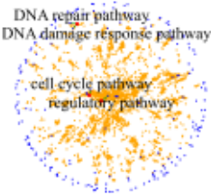
On the NS task, HIME significantly outperforms all other methods. Specifically, it outperforms Poincar´e by 251%, 76% and 132% on the three datasets. Besides, there exists a positive correlation between HIME's performance and K, since the node-label distances of positive pairs will decrease when the underfitting problem is alleviated by large K, as illustrated by the small node-label distances between gene OR7G3 and its pathways in the Poincar´e ball shown in figure 3. Furthermore, all the branch vectors are uniformly distributed in the whole Poincar´e ball, reducing the density of branch vectors around a given label and leading to a more accurate node search near the label. By contrast, the branch vectors and the labels in EUHIME are embedded into two separate groups due to its score function and the negative sampling, making it hard for EUHIME to correctly search the label's true branch vectors from a crowd of wrong ones.
| Protein-GO | Gene-Pathway | DBLP-ACM | ||||||||||
|---|---|---|---|---|---|---|---|---|---|---|---|---|
| Method | LS | NS | CS | HC | LS | NS | CS | HC | LS | NS | CS | HC |
| Node2Vec | 85.29 | 18.32 | 72.93 | 10.31 | 79.81 | 47.51 | 73.27 | 23.76 | 59.09 | 12.57 | 71.38 | 18.32 |
| GraphGAN | 75.01 | 25.58 | 70.33 | 11.43 | 62.82 | 28.18 | 78.23 | 20.73 | 69.36 | 33.15 | 71.29 | 13.01 |
| GraphSAGE | 71.58 | 23.69 | 73.13 | 8.70 | 49.11 | 15.64 | 76.77 | 21.41 | 77.03 | 26.33 | 69.59 | 36.21 |
| PTE | 55.71 | 19.53 | 63.65 | 8.64 | 47.09 | 34.36 | 59.69 | 28.05 | 49.51 | 13.07 | 46.00 | 12.91 |
| JOIE | 87.81 | 28.46 | 79.87 | 14.84 | 63.10 | 32.50 | 75.74 | 29.10 | 67.10 | 25.34 | 70.00 | 17.83 |
| TaxoGAN | 43.55 | 4.55 | 51.73 | 61.31 | 58.23 | 6.10 | 50.17 | 41.15 | 53.09 | 4.90 | 48.95 | 43.38 |
| Poincare | 92.54 | 22.25 | 88.88 | 18.07 | 86.23 | 54.96 | 81.77 | 22.31 | 82.04 | 39.12 | 69.70 | 25.19 |
| Lorentz | 93.07 | 25.75 | 89.29 | 22.88 | 89.22 | 52.42 | 82.13 | 19.50 | 85.18 | 41.10 | 71.01 | 29.89 |
| HIME 2 | 97.70 | 48.48 | 90.19 | 53.89 | 95.85 | 88.18 | 85.65 | 37.14 | 96.05 | 85.03 | 81.90 | 51.48 |
| HIME 4 | 97.86 | 70.55 | 88.94 | 47.88 | 96.07 | 93.52 | 85.44 | 55.84 | 96.92 | 89.19 | 82.18 | 55.42 |
| HIME 8 | 98.02 | 78.17 | 89.08 | 51.77 | 95.91 | 96.85 | 85.93 | 55.02 | 96.93 | 90.98 | 82.07 | 57.73 |
| EUHIME 8 | 98.56 | 59.90 | 86.58 | 60.84 | 94.24 | 22.31 | 78.11 | 69.06 | 94.09 | 23.89 | 53.08 | 62.02 |
| Protein-GO | Gene-Pathway | DBLP-ACM | ||||
|---|---|---|---|---|---|---|
| Method | PRC | ROC | PRC | ROC | PRC | ROC |
| Node2Vec | 62.65 | 79.26 | 36.13 | 66.19 | 53.28 | 69.96 |
| GraphGAN | 74.11 | 85.64 | 41.58 | 74.96 | 62.66 | 74.47 |
| GraphSAGE | 48.60 | 72.33 | 27.03 | 56.09 | 35.17 | 60.37 |
| PTE | 69.87 | 83.16 | 33.03 | 68.03 | 41.98 | 68.69 |
| JOIE | 70.44 | 83.28 | 35.10 | 65.99 | 42.49 | 66.30 |
| TaxoGAN | 73.97 | 85.56 | 40.62 | 73.63 | 63.19 | 73.26 |
| Poincare | 72.18 | 85.13 | 39.84 | 73.46 | 60.43 | 74.32 |
| Lorentz | 74.19 | 85.53 | 36.17 | 69.99 | 58.31 | 73.10 |
| HIME 2 | 80.88 | 88.95 | 45.73 | 75.70 | 68.80 | 78.23 |
| HIME 4 | 82.93 | 89.10 | 45.68 | 76.88 | 70.79 | 79.16 |
| HIME 8 | 81.99 | 89.13 | 47.54 | 77.08 | 71.01 | 79.04 |
| EUHIME 8 | 79.22 | 88.65 | 46.16 | 76.75 | 66.37 | 78.22 |
| RHIME 8 | 70.22 | 83.65 | 39.25 | 74.39 | 63.10 | 75.80 |
On the CS task, HIME and Lorentz are the two best methods, followed by Poincar´e and JOIE. These methods preserve the parent-child relationships by either defining an asymmetric score for the directed relationships or generating a more hierarchical embedding in hyperbolic spaces. Compared with HIME, EUHIME is less capable of generating an accurate taxonomy in Euclidean space, especially on DBLPACM with dense node-label links which dilute the effect of its symmetric label refinement on the label vectors.
Hierarchical Classification
Given a node, Hierarchical Classification (HC) is to predict a correct label path with the knowledge of the taxonomy. Starting from the root label, if a label is correctly predicted from its siblings, then the classification will continue to its child labels, otherwise it will stop. Acc is computed for each node as the ratio of the accurate predicted labels to the whole labelpath. Acc evaluates the performance on all nodes.
On the HC task, EUHIME, HIME and TaxoGAN are the three leading methods.The good performance of TaxoGAN on HC is mainly due to the fact that it is specialized in predicting a node's label from the label's siblings by embedding them into a separate space. This ensures a more precise embedding but also sacrifices the universality of the vectors, which accounts for its notably poor performance on NS. Surprisingly, EUHIME is more capable than HIME of predicting a correct label path for a node, which can be explained by its inner-product score function: a branch vector can simultaneously increase the inner-product scores of all the labels in a path by increasing its norm or decreasing the angle to the label's directions. However, EUHIME also fails on the NS tasks as discussed before. Besides, its embedding provides less visual information compared with HIME that optimizes vectors according to their space distances.
Link Prediction
Link prediction tests a method's ability to predict potential node-node links. A method predicts unseen links from the negative ones by ranking the scores of node pairs. AUPRC and AUROC are calculated to evaluate the ranking.
Table 3 displays the results on link prediction. HIME has the highest AUPRC and AUROC compared with other methods, with EUHIME being the second and GraphGAN the third. RHIME has a relatively poor performance compared with HIME, indicating the effectiveness of using label information in predicting node-node links. Although the node vectors in other methods also contain label information, the abundant node-label links actually impose burdens on the node vectors other than providing information for predicting unseen node-node links, while these burdens are taken off by the multiple branch vectors in HIME.
6 Conclusions
The extensive experiments show the outstanding performance of HIME compared with existing methods. The ablation studies reveal the effectiveness of the Poincare ball in preserving the hierarchical taxonomy and the usefulness of branchdependent root vectors in preserving the network proximity. HIME can be easily extended to diverse manifolds by equipping different distance functions. Techniques used by traditional methods such as random walks on meta-paths can be also applied by HIME.
Acknowledgments
We acknowledge the support by the High-Performance Computing Platform of Peking University, Beijing, China.
@inproceedings{ijcai2022p408,
  title     = {Multi-Vector Embedding on Networks with Taxonomies},
  author    = {Fan, Yue and Ma, Xiuli},
  booktitle = {Proceedings of the Thirty-First International Joint Conference on
               Artificial Intelligence, {IJCAI-22}},
  publisher = {International Joint Conferences on Artificial Intelligence Organization},
  editor    = {Luc De Raedt},
  pages     = {2944--2950},
  year      = {2022},
  month     = {7},
  note      = {Main Track},
  doi       = {10.24963/ijcai.2022/408},
  url       = {https://doi.org/10.24963/ijcai.2022/408},
}
TY - CPAPER TI - Multi-Vector Embedding on Networks with Taxonomies AU - Fan, Yue AU - Ma, Xiuli T2 - Proceedings of the Thirty-First International Joint Conference on Artificial Intelligence, IJCAI-22 PB - International Joint Conferences on Artificial Intelligence Organization PY - 2022 SP - 2944 EP - 2950 DO - 10.24963/ijcai.2022/408 UR - https://doi.org/10.24963/ijcai.2022/408 ER -Copied
Machine-readable versions of this paper, for tools and AI agents:





