
Memory Augmented State Space Model for Time Series Forecasting
Proceedings of the Thirty-First International Joint Conference on Artificial Intelligence. Main Track. Pages 3451-3457.
https://doi.org/10.24963/ijcai.2022/479
Keywords
- Machine Learning: Time-series; Data Streams
- Machine Learning: Probabilistic Machine Learning
- Uncertainty in AI: Inference
- Machine Learning: Bayesian Learning
Abstract
State space model (SSM) provides a general and flexible forecasting framework for time series. Conventional SSM with fixed-order Markovian assumption often falls short in handling the long-range temporal dependencies and/or highly non-linear correlation in time-series data, which is crucial for accurate forecasting. To this extend, we present External Memory Augmented State Space Model (EMSSM) within the sequential Monte Carlo (SMC) framework. Unlike the common fixed-order Markovian SSM, our model features an external memory system, in which we store informative latent state experience, whereby to create ``memoryful" latent dynamics modeling complex long-term dependencies. Moreover, conditional normalizing flows are incorporated in our emission model, enabling the adaptation to a broad class of underlying data distributions. We further propose a Monte Carlo Objective that employs an efficient variational proposal distribution, which fuses the filtering and the dynamic prior information, to approximate the posterior state with proper particles. Our results demonstrate the competitiveness of forecasting performance of our proposed model comparing with other state-of-the-art SSMs.
- [Alaa and van der Schaar, 2019] Ahmed M Alaa and Mi- haela van der Schaar. Attentive state-space modeling of disease progression. Advances in Neural Information Pro- cessing Systems, 32:11338-11348, 2019.
- [Arasaratnam and Haykin, 2009] Ienkaran Arasaratnam and Simon Haykin. Cubature kalman filters. IEEE Transac- tions on automatic control, 54(6):1254-1269, 2009.
- [Bauwens et al., 2006] Luc Bauwens, Sébastien Laurent, and Jeroen VK Rombouts. Multivariate garch models: a survey. Journal of applied econometrics, 21(1):79-109, 2006.
- [Bialek et al., 2001] William Bialek, Ilya Nemenman, and Naftali Tishby. Predictability, complexity, and learning. Neural computation, 13(11):2409-2463, 2001.
- [Blei et al., 2017] David M Blei, Alp Kucukelbir, and Jon D McAuliffe. Variational inference: A review for statisti- cians. Journal of the American statistical Association, 112(518):859-877, 2017.
- [Bošnjak et al., 2017] Matko Bošnjak, Tim Rocktäschel, Ja- son Naradowsky, and Sebastian Riedel. Programming with a differentiable forth interpreter. In International confer- ence on machine learning, pages 547-556. PMLR, 2017.
- [Chung et al., 2015] Junyoung Chung, Kyle Kastner, Lau- rent Dinh, Kratarth Goel, Aaron C Courville, and Yoshua Bengio. A recurrent latent variable model for sequential data. Advances in neural information processing systems, 28:2980-2988, 2015.
- [Dinh et al., 2016] Laurent Dinh, Jascha Sohl-Dickstein, and Samy Bengio. Density estimation using real nvp. arXiv preprint arXiv:1605.08803, 2016.
- [Fraccaro et al., 2016] Marco Fraccaro, Søren Kaae Sønderby, Ulrich Paquet, and Ole Winther. Sequential neural models with stochastic layers. arXiv preprint arXiv:1605.07571, 2016.
- [Fraccaro et al., 2017] Marco Fraccaro, Simon Kamronn, Ulrich Paquet, and Ole Winther. A disentangled recogni- tion and nonlinear dynamics model for unsupervised learn- ing. Advances in Neural Information Processing Systems, pages 3604--3613, 2017.
- [Gemici et al., 2017] Mevlana Gemici, Chia-Chun Hung, Adam Santoro, Greg Wayne, Shakir Mohamed, Danilo J Rezende, David Amos, and Timothy Lillicrap. Gen- erative temporal models with memory. arXiv preprint arXiv:1702.04649, 2017.
- [Gordon et al., 1993] Neil J Gordon, David J Salmond, and Adrian FM Smith. Novel approach to nonlinear/non- gaussian bayesian state estimation. In IEE Proceedings F-radar and signal processing, volume 140, pages 107- 113. IET, 1993.
- [Karl et al., 2016] Maximilian Karl, Maximilian Soelch, Justin Bayer, and Patrick Van der Smagt. Deep variational bayes filters: Unsupervised learning of state space models from raw data. arXiv preprint arXiv:1605.06432, 2016.
- [Kitagawa, 1996] Genshiro Kitagawa. Monte carlo filter and smoother for non-gaussian nonlinear state space models. Journal of computational and graphical statistics, 5(1):1- 25, 1996.
- [Krishnan et al., 2015] Rahul G Krishnan, Uri Shalit, and David Sontag. Deep kalman filters. arXiv preprint arXiv:1511.05121, 2015.
- [Krishnan et al., 2017] Rahul Krishnan, Uri Shalit, and David Sontag. Structured inference networks for nonlin- ear state space models. In Proceedings of the AAAI Con- ference on Artificial Intelligence, volume 31, 2017.
- [Kumar et al., 2016] Ankit Kumar, Ozan Irsoy, Peter On- druska, Mohit Iyyer, James Bradbury, Ishaan Gulrajani, Victor Zhong, Romain Paulus, and Richard Socher. Ask me anything: Dynamic memory networks for natural lan- guage processing. In International conference on machine learning, pages 1378-1387. PMLR, 2016.
- [Le et al., 2017] Tuan Anh Le, Maximilian Igl, Tom Rain- forth, Tom Jin, and Frank Wood. Auto-encoding sequen- tial monte carlo. arXiv preprint arXiv:1705.10306, 2017.
- [Lütkepohl, 2005] Helmut Lütkepohl. New introduction to multiple time series analysis. Springer Science & Business Media, 2005.
- [Maddison et al., 2017] Chris J Maddison, John Lawson, George Tucker, Nicolas Heess, Mohammad Norouzi, An- driy Mnih, Arnaud Doucet, and Yee Teh. Filtering vari- ational objectives. Advances in Neural Information Pro- cessing Systems, 30, 2017.
- [Naesseth et al., 2018] Christian Naesseth, Scott Linderman, Rajesh Ranganath, and David Blei. Variational sequential monte carlo. In International conference on artificial in- telligence and statistics, pages 968-977. PMLR, 2018.
- [Rasul et al., 2020] Kashif Rasul, Abdul-Saboor Sheikh, Ingmar Schuster, Urs Bergmann, and Roland Voll- graf. Multivariate probabilistic time series forecast- ing via conditioned normalizing flows. arXiv preprint arXiv:2002.06103, 2020.
- [Rasul et al., 2021] Kashif Rasul, Calvin Seward, Ingmar Schuster, and Roland Vollgraf. Autoregressive denoising diffusion models for multivariate probabilistic time series forecasting. arXiv preprint arXiv:2101.12072, 2021.
- [Salinas et al., 2019] David Salinas, Michael Bohlke- Schneider, Laurent Callot, Roberto Medico, and Jan Gasthaus. High-dimensional multivariate forecasting with low-rank gaussian copula processes. arXiv preprint arXiv:1910.03002, 2019.
- [Sukhbaatar et al., 2015] Sainbayar Sukhbaatar, Arthur Szlam, Jason Weston, and Rob Fergus. End-to-end memory networks. arXiv preprint arXiv:1503.08895, 2015.
- [Wen et al., 2022] Qingsong Wen, Tian Zhou, Chaoli Zhang, Weiqi Chen, Ziqing Ma, Junchi Yan, and Liang Sun. Transformers in time series: A survey. arXiv preprint arXiv:2202.07125, 2022. IJCAI
- [Weston et al., 2015] Jason Weston, Sumit Chopra, and An- toine Bordes. Memory networks. International Confer- ence on Learning Representations (ICLR), 2015.
References were extracted automatically from the PDF and may contain errors.
Full text extracted automatically from the PDF; figures, tables and equations may differ. The PDF is the version of record.
1 Introduction
Time series forecasting is vitally important in real world application, such as demand forecasting, optimizing business processes and financial risk management. One popular probabilistic time series forecasting framework is the state space models (SSM), whose key idea is to create a generative model of the data in terms of latent variables that captures the temporal evolution of the system (i.e., state transitions) , in comparison with many other non-generative models, such as Transformers [Wen et al., 2022], that normally require a lot of training data. The prediction of the observations can be obtained by the state's posterior estimation of the previous time step and the dynamic model of the state. SSMs are flexible for complex data patterns and are scalable to large datasets, while not accumulating errors as autoregressive models for multi-step forecasting.
One main challenge of SSM is its inference method. Specifically, for Linear Guassian SSM, straight-forward algorithms, such as Kalman Filter (KF), can be used to accurately infer the posterior state, but for other non-linear SSM, many early methods suffer from scalability problem, which leads to the development of the following methods to approximate the posterior distribution more efficiently: i) Variational Inference (VI); ii) Sequential Monte Carlo (SMC) or particle filters using weighted particles iii) Variational Sequential Monte Carlo (VSMC), combining VI and SMC, which is more flexible, accurate and more efficient, allowing increased number of particles.
Another challenge of SSM is the transition dynamics. The canonical SSMs follow the assumption of fixed-order k Markovian state transition, such as KF and other non-linear extensions, which is insufficient to characterize many systems of practical relevance. The failure of fixed-order Markovian state dynamics to learn long correlation or to model complex state dynamics quantitatively [Bialek et al., 2001] leads to the following VI-based SSM works. [Alaa and van der Schaar, 2019] applies attention mechanism into the SSM to model disease progression. [Chung et al., 2015] (variational recurrent neural network, VRNN), [Fraccaro et al., 2016] (stochastic recurrent neural network, SRNN), and [Krishnan et al., 2015] (Deep KFs) solve the non-fixed-order Markovian problems with gating mechanism, such as Long Short-Term Memory (LSTM) and Gate Recurrent Unit (GRU).
However, these non-fixed-order Markovian models for time series face a common challenge, i.e., the state transition dynamics is based on the historical context with finite length, suffering from the limited storage capacity of memorized history. We therefore propose the combination of memorybased non-fixed-order Markovian models and SMC to relieve this limitation, as SMC can achieve scalable state posterior estimation, fully utilizing the stochastic particles (samples), which to the best of our knowledge, has not been attempted.
To address these problems, we propose External Memory Augmented State Space Model (EMSSM), which provides multi-step ahead probabilistic forecast with non-Markovian state transition and does not accumulate prediction errors like autoregressive models [Rasul et al., 2020; Rasul et al., 2021; Salinas et al., 2019]. The prior transition of EMSSM is augmented with external memory network for efficient learning. Our external memory is designed to preserve not only the context window but all the historical states, while fusing the information with noisy particles. In addition, we incoporate VSMC [Naesseth et al., 2018] as the inference algorithm, and the accurate posterior state with weighted particles sampled by VSMC can be stored in the external memory. Furthermore, resorting to Normalizing Flows (NF) as the emission model, EMSSM can adapt to data of complex distributions and high-dimension.
In summary, the main contributions of this paper are the following:
- A novel external memory augmented SSM architecture equipped with conditional NF to forecast multivariate time series with high-dimensional complex data distribution, yielding competitive performances compared with other SSMs in real-world datasets
- The demonstration that external memory can efficiently utilize the weighted particles sampled by VSMC and can handle the long-term nonlinear temporal dependencies
- A powerful dynamic function better expressing partially predictable observations, contributing to lower KL divergence in comparison to other SSMs
The paper is organized as follows. We first illustrate the problem definition in Sec.2, and then we review the related literature in Sec.3. The generative and inference model are introduced in Sec.4. Experiment and Conclusion are presented in Sec 5, Sec.6, respectively.
2 ProblemDefinition
The general probabilistic time series forecasting problem is defined as follows. Let yt ∈ Rv and xt ∈ Rk denote the time series target, and the time-varying covariate (input) vector, repectively, at time t. SSM models the temporal correlations and long-term dependencies among observation vectors y1:T := [y1, y2, ..., yT ] via unobserved (latent) state representation z1:T := [z1, z2, ..., zT ], where z ∈ Rd . SSM is characterized by transition distribution zt ∼ p(zt|z<t, xt) = fθ(·|z<t, xt) and emission distribution yt ∼ p(yt|zt, xt) = gθ(·|zt, xt), where θ denotes the parameters of the generative model. The conditional transition density fθ(·|z<t, xt)) models the temporal dynamics of the system, which defines how the latent zt is updated given the input xt and the previous states z<t. The noisy observation variable yt is generated by the latent state zt via the emission density gθ(·|zt, xt), given the current state zt and input xt. Under the assumption of SSM and d-separation properties of the graphical model, the joint distribution p(y1:T , z1:T |x1:T ) can be factorized as:
3 RelatedWork
3.1 Inference of SSM
For linear Gaussian systems, Kalman Filter (KF) can be used to solve the inference problem analytically. In contrast, for non-linear SSM, the exact inference becomes intractable and many approximate algorithms have been proposed, which can be summarized as follows:
- The deterministic methods such as the extended KF and Variational Inference (VI) [Arasaratnam and Haykin, 2009; Blei et al., 2017]. These methods can quickly approximate the posterior state, but lack accuracy.
- The stochastic methods, such as particle filters or smoothers that approximate the exact posterior distributions using a set of weighted samples (particles) via sequential Monte Carlo [Gordon et al., 1993; Kitagawa, 1996], can get faithful posterior estimation, but suffer from inefficiency.
- The hybrid algorithms, such as stochastic VI [Krishnan et al., 2017; Karl et al., 2016] and variational SMC(VSMC) [Naesseth et al., 2018; Maddison et al., 2017; Le et al., 2017], can balance between efficiency and reliability of the posterior estimation, and here in this work, we adopt VSMC to approximate the posterior distribution using augmented proposal distribution in SMC with variational distribution.
3.2 Memory-based Approach for Complex System
Internal Memory. Constructing the well-defined transition dynamics for the state is vitally important in SSM. Conventional SSMs follow the fixed-order Markovian dynamic assumption, ignoring the long-term complex temporal dependencies. A lot of effort based on the VI framework has been devoted to overcome the flaw of this naive assumption. [Chung et al., 2015](variational recurrent neural network/VRNN), [Fraccaro et al., 2016](stochastic recurrent neural network/SRNN), [Krishnan et al., 2015](Deep KFs) utilize LSTM or GRU to model the state dynamics while preserving the information over long intervals. Such recurrent dynamics, integrating both the computation and the memory storage, can be regarded as internal memory, which has two major drawbacks, i.e., poor scalability and restricted capability to distill information over the context of limited length.
External Memory. External memory-augmented neural network (MANN) has been used to increase the network capacity and to better capture long-term structure within sequences. It was originally proposed in [Weston et al., 2015] and expanded in later works [Sukhbaatar et al., 2015]. The combination of memory buffer and differentiable addressing mechanism has been developed to alleviate the memory capacity constraint in several tasks such as natural language processing [Kumar et al., 2016; Sukhbaatar et al., 2015] and algorithm learning [Boˇsnjak et al., 2017].
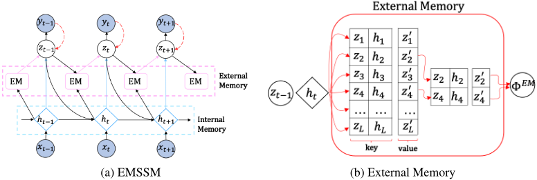
Motivated by the success of external memory in various areas, we incorporate the same mechanism into SSM to model the transition dynamics of time series, to address the limitation of internal memory. External memory here stores the accurate posterior state with weighted particles sampled by VSMC, which facilitates the main idea of our framework, i.e., similar target evolution over time corresponds to similar hidden states and the same target value will appear again with high probability. We will demonstrate later that the search and retrieval of similar posterior state preserved in external memory improves the forecasting performance.
.
4 Memory-Augmented State Space Model
In this section, we describe the proposed External Memory Augmented State Space Model (EMSSM), whose overall structure is illustrated in Figure 1. Unlike VRNN or SRNN, we add the additional dependency on the external memory when generating zt, and the whole memory architecture consists of internal memory and external memory listed below:
- Internal Memory corresponds to GRU network, distilling the information from local context window.
- External Memory memorizes the historical state transitions, which integrate information of the past states, covariates and targets, recording both the global temporal pattern ( which cannot be distilled from the local context window) and the stochastic part of p(zt|z<t, xt) in the past context. Figure 1(b) shows the schematics of External Memory.
4.1 Internal Memory
Internal memory is constructed with GRU network, which recursively preserves information into a vector with fixed size for later retrieval. Given the previous latent state vector zt-1 ∈ Rd , the previous hidden state ht-1 ∈ Rl , the covariate input xt and the multi-layer recurrent GRU network fGRU with parameter θ, at every time step, GRU updates the current hidden state ht and outputs the encoded dense vector ΦIM , which fuses the information from the local context:
Above RNN encoded context information is the major component proposed in VRNN and SRNN, with a major drawback that no global information is shared among different time windows. Especially for the historical latent states further away from the current window. For example, in the demand-forecasting scenario, the latent state of the same holiday last year may be an important reference of the demand estimation for the current year. To overcome the limitation of internal memory, we propose to use the additional external memory.
4.2 External Memory
Unlike the internal memory, the external memory with size L is a refreshed buffer, storing the historical posterior state transitions. The external memory distills the stochastic information of p(zt|z<t, xt) depending on noisy particles of zt which is conditioned on zt-1 and ht. The external memory consists of both key and value memories:
where zi ∈ Rd represents the previous state, hi is the GRU state, and z′i ∈ Rd represents the transitioned state.
In SSM, KL divergence KL(q(zt|xt, yt)|p(zt|zt-1, xt)) quantifies the additional information besides the prior knowledge over the latent state when predicting the current observation. KL divergence being zero means that the current observation can be well predicted by the prior information defined by the transition distribution alone. But the prior knowledge or the prior construction function generally does not have all the information, which contributes to the discrepancy between the real target and the prediction, e.g., forecasting the sales amount during promotions. To bridge the gap between the prior and the posterior, we employ external memory to record the historical state transitions, i.e., the non-parameterized distribution mapping M : zt-1 ↦-→ zt between the previous (zt-1) and the post latent states (zt). zt is obtained as the weighted average of all P particles from the sequential Monte Carlo (SMC) algorithm:
As a result of equation 3, we do not keep all the P particles {zpt }Pp=1 for computation efficiency and space saving purposes.
External Memory Controller. When training random sequences in every batch, the weighted latent state zt (equation 3) and hidden GRU state ht = ∑Pp=1 ωphpt form the state transition pair {[zt-1, ht], zt} that is written into the memory. To eliminate the information retrieval redundancy, we perform the state vector neighborhood subset generation
via the function fn(·) such as the kd-tree, cosine similarity, Euclidean distance, etc. Then to retrieve the memory vector, we use the function fw(·) to yield soft attention weights or the average weights wt.
Lastly, the retrieved external memory context ΦEM is a weighted sum of the row vectors of M sub v with weights wt:
The final memory output context Φt is the concatenation of the GRU output ΦIM obtained in equation 1 and the external memory output ΦEM obtained in equation 4:
which is then fed into the generative model in equation 6 below.
4.3 Generative Model
In the state space model, firstly we focus on the joint distribution of the latent states and observations which consists of the transition and emission distribution. The overall joint distribution in our EMSSM can be modeled via the following factorization:
where Φ1:T is the output of the external memory system defined in equation 5.
Transition Distribution. The transition distribution describes how the dynamic states zt evolve with the prior knowledge xt, andz<t. In the classic KF, the state zt has the linear map with covariate xt and the previous state zt-1. We adopt the external memory to model the state evolution to better capture the long-term dependency:
where zt-1 is the stochastic latent state, ht-1 is the deterministic hidden state of GRU and xt is the covariate. The transition density function fθ(·|Φt(zt-1, ht-1, xt)) is specified as a diagonal Gaussian distribution with mean and variance parameterized by the output of a multilayer perceptron (MLP) network by the memory context Φt using the reparameterization trick.
Emission Distribution. The emission model describes the time series data generation process. In order to adapt to high dimensional complex data distribution, we combine the multilayer perceptron transformation and conditional normalizing flow (CNF). The emission distribution is modeled by the following formula:
where the emission density function gθ(·|·) is a CNF transforming the base distribution N(0, I) to a complex target distribution. For NF, the base distribution p(X) can be mapped to the data distribution p(Y) via multiple coupling layers: X ↦→ C (0) ↦→ C (1) ↦→ · · · ↦→ C (n) ↦→ Y. The relation between the probability density (PDF) p(X) and p(Y) can be expressed by the change of variable formula: p(X) = p(Y) ∣∣det ( ∂Y ∂X )∣∣. We build our model block by adopting the non-volume preserving flow, such as RealNVP [Dinh et al., 2016] whose Jacobian determinant is a lower triangular matrix that can be efficiently computed. p(X) is chosen as the standard normal distribution X ∼ N(0, I) and the coupling layer output C (i) is conditioned on the latent state zt, which means the mapping varies with time via the CNF mechanism. The nonlinear transformation function hθ(zt) is implemented by multilayer perceptron (MLP) network with input zt.
4.4 Inference and Parameter Learning
Sequential Monte Carlo. Given the observations y1:T and covariates x1:T , we want to infer the posterior states z1:T and learn the parameter θ of the generative model for our dynamic SSM. To learn θ, one can maximize the marginal probabilistic density p(y1:T ) by integrating out z1:T :
However, the above integral cannot be carried out analytically because the generative and emission models are implemented with a neural network, for which we employ the technique of VI [Blei et al., 2017] to convert maximizing the marginal probabilistic density into maximizing the evidence lower bound (ELBO), using the concavity of log function and Jensen's inequality.
where qϕ(z1:T ) is taken from a family of distributions with parameter ϕ. Following the recent development of the Bayesian inference, we perform the variational sequential Monte Carlo (VSMC) algorithm with P particles [Naesseth et al., 2018], which uses the variational distribution as the proposal distribution. The algorithm gives an unbiased estimate of the marginal likelihood ˆ pθ(y1:T ) = ∏Tt=1 [1/P ∑Pp=1 ω(p) t ], where ω(p) t is the unnormalized importance weight of particle p at time t and maximize the surrogate ELBO
After training the objective, the proposal distribution for the inference is learned simultaneously. The biased gradient of surrogate ELBO ∇ ˜ F(θ, ϕ) ≈ Eε∼N(0,1)[∇log ˆ pθ,ϕ(y1:T )], omitting the score gradient term, is applied to maximize ˜ F(θ, ϕ), which leads to faster convergence as the prior and the posterior distributions are reparameterized with the parameters θ and ϕ.
Proposal Distribution. A good estimate with low variance using the SMC algorithm relies on the design of the proposal distribution. Our proposal distribution utilizes both the prior knowledge Φ of of the predictive prior dynamics in the generative model and the observation yt. The proposal distribution uses GRU as the base feature extraction network to learn the filter or smoothing posterior collecting the information in all time steps. The encoded feature at ∈ Rp is generated by passing the target value yt and covariate xt to the GRU network. The final proposal context Ψ is the concatenation of memory output context Φ and encoded feature at:
The inference density function fϕ(·|Ψ) is also specified as a diagonal Gaussian distribution whose mean and variance are parameterized by the output of a multilayer perceptron (MLP) and inference memory context Ψ using the reparameterization trick. Here, motivated by the work of [Fraccaro et al., 2016], rather than directly learning zt, we learn the residual term ˜zt between the true posterior zt and prior mean zprior,t, i.e., ˜zt = zt - zprior,t. Equivalently, the final posterior zt = ˜zt + zprior,t.
5 Experiment Results
5.1 EvaluationMetric and Data Set
We evaluate our model for multivariate time series forecasting on five popular public datasets including electricity, solar, traffic, exchange, and wikipedia (see [Rasul et al., 2020] for the properties and the summary of the datasets). These public datasets exhibit different seasonal patterns with hourly and daily frequencies. For the evaluation of different models, each dataset prior to the fixed forecast date is used as training data and the remaining data as the prediction data. The rolling window prediction starting from the fixed forecasting date is adopted as model evaluation method.
The continuous ranked probability score (CRPS) is a wellknown probabilistic model metric that measures the compatibility of model's cumulative distribution function (CDF) F of the observation y, defined as
where Iy≤u is the indicator function which is one if y ≤ u and zero otherwise. Lower CRPS scoring means better performance of the model's forecasting ability. The model's CDF can be approximated by the empirical CDF with n samples ˆ yi: ˆ F(u) = 1/n ∑ni=1 I{ˆ yi ≤ u}. However, the CRPS metric is defined for univariate time series, and it cannot capture the dependencies across different time series. Therefore, we use CRPSsum as the metric for multivariate time series forecasting, which can be obtained by first summing across different time series yielding CRPSsum = Et[CRPS( ˆ Fsum(t), ∑i xit )]. The CRPSsum metric has been theoretically and experimentally justified in the previous work.
5.2 Results
We compare our model with other SSMs (KAVE, VRNN, SRNN and Latent only model) and other multivariate time series forecasting model (GARCH, DeepVAR and GRU RealNVP). We also incorporated the same NF (RealNVP) to the original VRNN and SRNN models for a fair comparison and ablation study. The results are shown in Table 1 where the mean and standard errors are obtained by three independent runs.
- GARCH [Bauwens et al., 2006; L¨utkepohl, 2005] is a multivariate generalized autoregressive conditional heteroskedasticity model.
- DeepVAR lowrank-copula [Salinas et al., 2019] models the dynamics of the time series via the RNN and constructs the real data distribution via low-rank Gaussian copula.
- KVAE [Fraccaro et al., 2017] is a variational autoencoder structure combined with the linear Gaussian state space model to model the dynamics of the multivariate time series data.
- GRU RealNVP [Rasul et al., 2020] unrolls the GRU network describing the dynamics and model the complex data distribution via CNF.
- VRNN RealNVP uses the VRNN [Chung et al., 2015] to model the data dynamics and augment the emission distribution with CNF.
- SRNN RealNVP utilizes the SRNN [Fraccaro et al., 2016] to model the data dynamics and augment the emission distribution with CNF.
| Method | exchange | solar | electricity | traffic | wiki |
|---|---|---|---|---|---|
| GARCH | 0.023 ± 0.000 | 0.88 ± 0.002 | 0.19 ± 0.001 | 0.37 ±0.0016 | - |
| KAVE | 0.014 ± 0.002 | 0.34 ± 0.025 | 0.051 ±0.019 | 0.1±0.005 | 0.095 ± 0.012 |
| DeepVAR lowrank-Copula | 0.007 ±0.000 | 0.319±0.011 | 0.064 ±0.008 | 0.103 ±0.006 | 0.241 ±0.033 |
| GRU RealNVP | 0.0064 ± 0.001 | 0.331 ± 0.02 | 0.024 ±0.001 | 0.078 ±0.001 | 0.078 ±0.001 |
| VRNN RealNVP | 0.0072 ± 0.0004 | 0.416 ±0.011 | 0.027 ±0.003 | 0.062 ±0.002 | 0.070 ±0.002 |
| SRNN RealNVP | 0.0071 ± 0.0002 | 0.406 ±0.006 | 0.037 ±0.002 | 0.082 ±0.006 | 0.064 ±0.001 |
| Latent only RealNVP | 0.0074 ± 0.0005 | 0.412 ±0.008 | 0.034 ±0.003 | 0.105 ±0.002 | 0.065 ±0.001 |
| EMSSM RealNVP(ours) | 0.0059±0.0003 | 0.360 ±0.013 | 0.023±0.001 | 0.060±0.002 | 0.061±0.001 |
- Latent only RealNVP utilizes the latent only structure [Gemici et al., 2017] to model the data dynamics and augment the emission distribution by CNF. This structure can be seen as the variant of VRNN where the emission model only uses the latent variable without utilizing the RNN output. This model is evaluated for ablation purpose.
In Table 1, we observe that EMSSM with RealNVP achieves the state-of-the-art CRPSsum metric on 4 of the 5 datasets. In comparison against VRNN and SRNN, EMSSM demonstrates competitive forecasting capability, indicating the effectiveness of the external memory mechanism, which can be further verified by the ablation comparison study. Specifically, twomodel instances are compared, i.e., EMSSM with RealNVP against Latent only RealNVP that can be seen as EMSSM without the memory block. A lower CRPSsum from EMSSM demonstrates the advantage of using the memory. In addition, the competitive forecasting performance in the datasets of different strengths of seasonality further implies that our model can capture data pattern beyond seasonality. We omit further discussion due to space limitation.
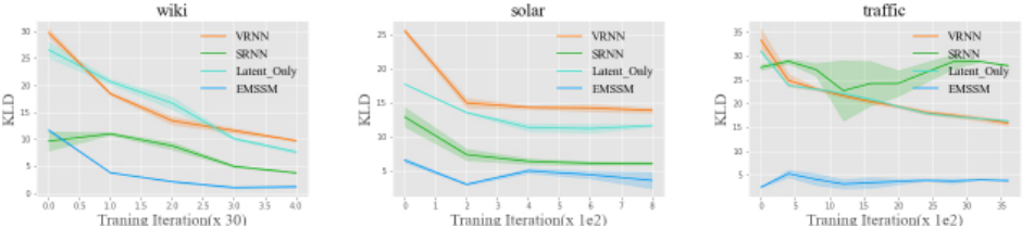
KL divergences per time-step over zt measure the additional information between the prior distribution and posterior distribution which is used to express the current observation. Lower KL divergences indicate that the prior function can explain most part of the current observation and the target is thus more predictable. Figure 2 shows the KL divergence of training sequence in the real-world datasets mentioned above, where we can see that using external memory yields almost the fastest drop and the lowest level of the KL divergence compared with other deep SSMs. This implies that the historical state information preserved in the external memory actually reduces the discrepancy between the prior and posterior distributions.
The time and space complexities of our EMSSMmodel are O(d2 + dl + dL)P T ) and O((d + l)(P T + L)), respectively, whereas the time and space complexities of VRNN/SRNN model are O((d2 + dl)PT ) and O((d + l)PT ), respectively, where we denote the time step as T, the number of particles as P, the dimension of hidden state ht of GRU as l, the dimension of latent state as d, and the buffer size of the external memory as L. Due to the additional external memory, our model has higher time and space complexities than VRNN/SRNN, but our model demonstrates faster convergence and smaller prediction error as shown in Figure 2.
6 Conclusion
In this paper, we proposed a memory-augmented state space model with CNF for multivariate time series forecasting, providing multi-step ahead probabilistic forecast with nonMarkovian state transition. The memory consists of both internal memory and external memory buffers, designed to memorize the global temporal pattern and the posterior state transitions, respectively. Our mechanism demonstrated lower KL divergence and better forecasting performance compared with other SSM models. The combination of CNF and the memory mechanism under the SSM framework enhanced the forecasting ability for multivariate time series in our experiments and we believe that our proposed method can better solve difficult real-world time series forecasting problems, such as holiday sales forecasting and anomaly detection, etc. For the future work, a more efficient storage and sampling mechanism for the memory buffer (e.g., using the information entropy) might further improve the training efficiency and prediction performance, which we will leave for further investigation.
@inproceedings{ijcai2022p479,
  title     = {Memory Augmented State Space Model for Time Series Forecasting},
  author    = {Sun, Yinbo and Ma, Lintao and Liu, Yu and Wang, Shijun and Zhang, James and Zheng, YangFei and Yun, Hu and Lei, Lei and Kang, Yulin and Ye, Llinbao},
  booktitle = {Proceedings of the Thirty-First International Joint Conference on
               Artificial Intelligence, {IJCAI-22}},
  publisher = {International Joint Conferences on Artificial Intelligence Organization},
  editor    = {Luc De Raedt},
  pages     = {3451--3457},
  year      = {2022},
  month     = {7},
  note      = {Main Track},
  doi       = {10.24963/ijcai.2022/479},
  url       = {https://doi.org/10.24963/ijcai.2022/479},
}
TY - CPAPER TI - Memory Augmented State Space Model for Time Series Forecasting AU - Sun, Yinbo AU - Ma, Lintao AU - Liu, Yu AU - Wang, Shijun AU - Zhang, James AU - Zheng, YangFei AU - Yun, Hu AU - Lei, Lei AU - Kang, Yulin AU - Ye, Llinbao T2 - Proceedings of the Thirty-First International Joint Conference on Artificial Intelligence, IJCAI-22 PB - International Joint Conferences on Artificial Intelligence Organization PY - 2022 SP - 3451 EP - 3457 DO - 10.24963/ijcai.2022/479 UR - https://doi.org/10.24963/ijcai.2022/479 ER -Copied
Machine-readable versions of this paper, for tools and AI agents:





