
Estimation and Comparison of Linear Regions for ReLU Networks
Proceedings of the Thirty-First International Joint Conference on Artificial Intelligence. Main Track. Pages 3544-3550.
https://doi.org/10.24963/ijcai.2022/492
Keywords
- Machine Learning: Theory of Deep Learning
- Machine Learning: Learning Theory
- Machine Learning: Optimisation
Abstract
We study the relationship between the arrangement of neurons and the complexity of the ReLU-activated neural networks measured by the number of linear regions. More specifically, we provide both theoretical and empirical evidence for the point of view that shallow networks tend to have higher complexity than deep ones when the total number of neurons is fixed. In the theoretical part, we prove that this is the case for networks whose neurons in the hidden layers are arranged in the forms of 1x2n, 2xn and nx2; in the empirical part, we implement an algorithm that precisely tracks (hence counts) all the linear regions, and run it on networks with various structures. Although the time complexity of the algorithm is quite high, we verify that the problem of calculating the number of linear regions of a ReLU network is itself NP-hard. So currently there is no surprisingly efficient way to solve it. Roughly speaking, in the algorithm we divide the linear regions into subregions called the "activation regions", which are convex and easy to propagate through the network. The relationship between the number of the linear regions and that of the activation regions is also discussed.
- [Google, 2016] Google. Tensorflow playground. https:// playground.tensorflow.org/, 2016. Accessed: 2022-05-08. Link
- [Hanin and Rolnick, 2019a] Boris Hanin and David Rolnick. Complexity of linear regions in deep networks. Interna- tional Conference on Machine Learning (ICML), 2019.
- [Hanin and Rolnick, 2019b] Boris Hanin and David Rolnick. Deep relu networks has surprisingly few activation pat- terns. Neural Information Processing Systems (NIPS), 2019.
- [Hunter et al., 2012] David Hunter, Hao Yu, Michael S. Puk- ish, Janusz Kolbusz, and Bogdan M. Wilamowski. Selec- tion of proper neural network sizes and architectures-a comparative study. IEEE Transactions on Industrial In- formatics, 8(2):228-240, 2012.
- [LeCun et al., 2010] Yann LeCun, Corinna Cortes, and CJ Burges. MNIST handwritten digit database. ATT Labs [Online]. Available: http://yann.lecun.com/exdb/mnist, 2, 2010. Link
- [Lei et al., 2020] Na Lei, Zhongxuan Luo, Shing-Tung Yau, and David Xianfeng Gu. Geometric understanding of deep learning. Engineering, 2020.
- [Montúfar et al., 2014] Guido Montúfar, Razvan Pascanu, Kyunghyun Cho, and Yoshua Bengio. On the number of linear regions of deep neural network. Neural Information Processing Systems (NIPS), 2014.
- [Raghu et al., 2017] Maithra Raghu, Ben Poole, Jon Klen- berg, Surya Ganguli, and Jascha Sohl Dickstein. On the expressive power of deep neural networks. International Conference on Machine Learning (ICML), 2017.
- [Serra et al., 2018] Thiago Serra, Christian Tjandraatmadja, and Srikumar Ramalingam. Bounding and counting linear regions of deep neural networks. International Conference on Machine Learning (ICML), 2018.
- [Sopena et al., 1999] Josep M. Sopena, Enrique Romero, and René Alquezar. Neural networks with periodic and monotonic activation functions: a comparative study in classification problems. Ninth International Conference on Artificial Neural Networks (ICANN 99), 1999.
- [Xiong et al., 2020] Huan Xiong, Lei Huang, Mengyang Yu, Li Liu, Fan Zhu, and Ling Shao. On the number of linear regions of convolutional neural networks. International Conference on Machine Learning (ICML), 2020.
References were extracted automatically from the PDF and may contain errors.
Full text extracted automatically from the PDF; figures, tables and equations may differ. The PDF is the version of record.
1 Introduction
In recent years, there has been increasing interest in exploring the inner structure of neural networks. Due to the fact that the ReLU activation function
is a piecewise linear function, the output of the whole network, viewed as a function of the input variable, is piecewise linear as well. In particular, the function naturally divide the input space into regions which are commonly referred to as "linear regions".
The behavior of the linear regions of a ReLU network has been studied by many approaches. In particular, many papers have estimated the number of the linear regions, such as [Mont´ufar et al., 2014; Raghu et al., 2017; Serra et al., 2018; Hanin and Rolnick, 2019a; Hanin and Rolnick, 2019b; Xiong et al., 2020]. However, a direct estimation on the expected number of linear regions is still far from ideal. Among the estimations so far, those in [Raghu et al., 2017] and [Hanin and Rolnick, 2019a] are about 1-dimensional trajectories through the linear region, and those in [Hanin and Rolnick, 2019b] are on activation patterns.
In this paper, aiming at the linear regions directly, we mainly discuss the influence of arrangement of neurons on them. According to both theoretical and empirical evidence discovered, we put forward the following
Claim 1: Generally speaking, for a ReLU-activated network, suppose that the total number of neurons in the hidden layers is fixed and the numbers of neurons in different layers are similar. When the weights and biases are randomly chosen, more linear regions are expected to be generated by shallow network than deep network.
This claim may not sound so surprising, because by easy calculation one can see that, when the total number of hidden neurons are fixed, shallow networks usually have more weights than deep ones, and that may result in the shallow networks having more linear regions. However, due to the complexity of the network structures, such relationship is not so easy to show. For example, in order to prove it theoretically, without being able to provide precise values, one needs to find a lower bounds for the expected number of linear regions of shallow networks and an upper bound for that of deep networks, such that the lower bound is greater than the upper bound. This requires a more delicate estimation for the number of linear regions, and the author is not aware of any result of this kind.
An easy case that one can immediately figure out though is that there is only one hidden layer in the network containing n neurons. In this case, each neuron in the hidden layer forms a hyperplane w · x + b = 0, where x is the input variable, w is the vector of weights toward the neuron and b is the bias. Then the linear regions associated with this neuron are the two half-spaces divided by this hyperplane. Denote the input dimension by M. If the hyperplanes for all the neurons in the hidden layer are in generic position (which happens with probability 1 when the weights and biases are sufficiently random), the number of linear regions in the output layer is
Especially when M ≥ n, this is 2n which is the theoretical maximum among all the arrangements of the neurons (see for example [Lei et al., 2020, Theorem 4.5]). However, in general the situation can be very complicated.
In this paper, we show that gaps for the expectation of the number of linear regions exist for ReLU-activated networks with hidden neurons arranged like 1×2n, 2×n and n×2. The statement of the theorem seems sufficiently concise, intuitive and self-contained so that we believe it can be directly put here in the introduction section as follows.
Theorem 1.1. Let N be a fully-connected ReLU-activated neural network whose weights and biases are all independent continuous random variables with even density functions. Suppose that the input dimension of N is M and the output dimension is 1. Define E(N) as the expectation of the linear regions resulting from N with respect to the weights and biases. We use Nk×l to indicate that N has l hidden layers and each of the hidden layer has k neurons. Then for all M ≥ 2 and n ≥ 1, E(N2×n) > E(N1×2n); for all M ≥ n and n ≥ 9, E(Nn×2) > E(N2×n).
We also put a complete version of Theorem 1.1 as Theorem 2.1. Theorem 2.1 reveals more technical details about the estimation of E(N), and Theorem 1.1 follows from it. The proofs of Theorem 2.1 and Theorem 1.1 are in the appendix which is in the supplementary material.
Besides 1.1, to support Claim 1, we implement an algorithm which tracks every linear region in detail, including the shape of the region and the value of the corresponding piecewise linear function on it. We run experiments with this algorithm on networks of small scale and calculate the number of linear regions directly. Among the network structures, there are the ones with different layers but the same number of weights and biases (see the second part of Section 4.1). The results we get from all the networks support the claim statistically (especially for cases where Theorem 1.1 does not cover).
It is worth pointing out that the algorithm is not completely new, as the rationale behind it has already been pointed out in [Raghu et al., 2017, Theorem 2]. The idea is to divide the linear regions into (convex) activation regions which are easy to track through the network. Still, we describe the algorithm from a more engineering perspective, including the procedures of generating each linear region reflected in our code and some optimization techniques therein. Some settings in the algorithm are also used in the proof of Theorem 1.1. Moreover, in the hope of illustrating and exploring more about the relationships between the linear regions and the activation regions, we provide a way to construct networks of arbitrary depth and various structures and parameters where the linear regions are exactly the same as the activation regions (see Theorem 3.1).
Our algorithm of finding linear regions is expected to have very high time and space complexity, and for this reason we find it unrealistic to run the algorithm for networks of very large scale. In fact, in this paper we verify that the problem of counting the linear regions for a ReLU-activated network is NP-hard (see Theorem 3.2), thus implying that a polynomialtime solution to the problem is extremely difficult to find.
Another natural question is whether the Claim 1 still holds in the process of training ReLU-activated networks. Due to the complexity and diversity of the training tasks in reality, it is very hard to give a uniform answer for this question. Nevertheless, we do an experiment for the well known two-spiral data in Section 4. There we can see that in this particular training task, for networks during the training process, the number of linear regions tends to decrease for shallow networks and increase for deep networks compared to the mean value when the parameters are completely random, but such change is too small to close the gap.
For the rest of the paper, we assume that every network we consider is activated by the ReLU function (1.1), and the output layer of it has only one neuron.
2 Estimation of the Number of Linear Regions
In this section, we present all the estimation results on the number of linear regions that we have obtained as follows.
Theorem 2.1. Let N be a fully-connected ReLU-activated neural network whose weights and biases are all independent continuous random variables with even density functions. Suppose that the input dimension of N is M and the output dimension is 1. Define E(N) as the expectation of the linear regions resulting from N with respect to the weights and biases.
- Suppose that N has n hidden layers, each having 1 neuron, and M ≥ 1. Then
- Suppose that N has 2 hidden layers, the first and the second layer has n1 and n2 neurons respectively, and M ≥ max(n1, n2). Define K(n1, n2) as
Then
- Suppose that N has n hidden layers (n ≥ 2), each having 2 neuron, and M ≥ 2. Then
When n1 and n2 are sufficiently large and are similar to each other, 2n1 is actually very small compared to K(n1, n2). So Part 2 restricts the number of linear regions for networks with 2 hidden layers to a quite narrow range. The techniques used in the proof for each part of Theorem 2.1 are of quite different styles. Roughly speaking, for Part 1, we formulate the number of linear regions for N as a 3-state random walk and analyze the transition matrix of it to find an upper bound for E(N). For Part 2, we consider the exact position of each hyperplane induced in each layer and figure out how many new distinct activation regions they are expected to generate from the activations in the previous layer. For Part 3, for the inequality on the left we find a lower bound for E(N) by analyzing the probability that a linear region that has nonzero slope and extends to infinity exists; for the equality on the right we consider the different cases for the hyperplanes generated in each neuron, and estimate the maximum multiples it can bring to E(N), and then combine this with the probability of dropout for each neuron to get the final upper bound.
3 Algorithm of Finding Linear Regions
We follow [Mont´ufar et al., 2014, Section 2.1] for the definition of linear region of a piecewise linear function, which is defined as a maximal connected subset of the input space on which the function is linear. Since the output of each neuron in a ReLU-activated network is a piecewise-linear function with respect to the input, there are the linear regions for it which we call the linear regions for that particular neuron. As a linear region is not necessarily convex, it is not quite easy to handle. Our strategy is to divide each linear region into convex regions shaped by hyperplanes, and group up these convex regions that are adjacent to each other and have common values to form the linear regions. Within each neuron, the convex regions from the neurons in the previous layer are intersected with each other and then cut into multiple convex regions of the through activation. We call such a convex region together with the value of the linear function on it an activation region. More specifically, an activation region consists of the following two parts:
- The shape, which is the region in the input space shaped by the restrictions
where r is the number of restrictions. It is easy to see that the region bounded by such a group of restrictions is convex, although not necessarily bounded. For an activation region c, we denote the shape of it by S(c).
- The value, which is a vector (v1, v2, ..., vM, t) representing the function v1x1 + v2x2 + ... + vMxM + t on the input space. For an activation region c, we denote the value of it by V (c).
We then define the following operations on activation regions:
- Intersection: for a list of activation regions c1, c2, ..., ck, if ⋂ki=1 S(ci) ̸= ∅, we define the intersection of c1, c2, ..., ck with coefficients w1, ...,wk to be a new activation region c such that S(c) = ⋂ki=1 S(ci), and V (c) = ∑ki=1 wiV (ci). This operation is denoted as c = Intersect(c1, ..., ck,w1, ...,wk). Note that in order to find ⋂ki=1 S(ci), we only need to put restrictions for all the ci's together, then check whether such group of restriction is valid and remove the redundant ones. In practice, we use linear programming to check the validity of the restrictions and to test whether each restriction is redundant.
- Addition: for an activation region c and a real number b, the addition operation simply change the value of c from (v1, v2, ..., vn, t) to (v1, v2, ..., vn, t + b). Such an addition operation is denoted as Add(c, b).
- Cut: for an activation region c, let V (c) = (v1, v2, ..., vn, t). We construct two activation regions via the cut operation. For the first activation region c1, S(c1) is formed by adding the restriction v1x1 +v2x2 + ... + vnxn + t ≤ 0 to S(c) and V (c1) is the zero vector. For the second activation region c2, S(c2) is formed by adding the restriction -v1x1-v2x2-...-vnxn-t ≤ 0 to S(c) and V (c2) = V (c). Finally we only keep the activation regions whose shapes are non-empty from c1 and c2. Intuitively, the cut operation is to apply ReLU based on V (c). We denote the cut operation as Cut(c).
With the definition of activation region and the operations at hand, we are ready to construct the activation regions for all layers inductively. Denote the number of neurons in the i-th hidden layer by ni, the input dimension by M, and the j-th neuron in the i-th layer by N i j . Denote the weights from the j-th neuron in the (i - 1)-th layer to the k-th neuron in the i-th layer by iwjk, and denote the bias for the k-th neuron in the i-th layer by i bk. In the first hidden layer, for the k-th neuron, there are two activation regions c1 and c2 shaped by the hyperplane ∑Mj=1 1wjkxj +1 bk = 0, where
Now suppose the activation regions for all neurons in the (i - 1)-th hidden layer is already constructed. Then for each neuron N i j in the i-th hidden layer, we enumerate all the combinations of activation regions c1, c2, ..., cni-1 where ck is an activation region of N i-1 k for all i. For each of such combination, we collect the (one or two) activation regions from
and all such activation regions are the activation regions for N i j . In other words, (3.2) distributes the operation of taking weighted sum (with bias) and applying the ReLU activation to all the activation regions in the form of the intersection of c1, c2, ..., cni-1 , and the results are also in the format of activation region. Therefore, by induction such construction can go through the whole network.
Finally, for the (only) neuron in the output layer, we still apply (3.2) for activation regions collected from the last hidden layer, but without the Cut part because there is no activation in the output layer. Then in order to find linear regions, we just need to group together those activation regions that are connected to each other and have the same value, and the number of such groups is the number of linear regions.
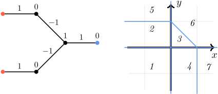
A simple example is given as Figure 1.
y
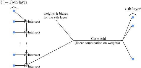
The original Intersection function requires that all the combination of activation regions from the previous layer are considered, so it definitely has very high complexity. In practice, to construct the activations for neurons in the i-th layer from those in the (i - 1)-th layer, we first do pairwise Intersection operation for the activation regions for the first and the second neurons in the (i - 1)-th layer and get a list of activation regions, and then do pairwise Intersection for this intermediate list of activation regions and the activation regions for the third neuron in the layer, and repeat this process until finishing with the last neuron in the layer. It is worth mentioning that the value part in an intermediate activation region is actually a list of values instead of a single value. For each pairwise Intersection of an intermediate activation region and an activation region in the next neuron in the layer, the shapes of activation regions are intersected, but the value of the new activation regions is appended to the list of values. In this way, after we are done with the last neuron in the (i - 1)-th layer, the shape of an activation region c in the intermediate neuron is still of the same form as in 1, but the value of c is of the form (u1, u2, ..., uni-1 ), where each ui is a vector of length M. Then for the k-th neuron in the i-th layer, we take weighted sum for the values as ∑ni-1 l=0 iwlkul to form the value for c which matches the form in 2, and then perform the Add and Cut operations for each c to finally get all the activation regions for the corresponding neuron. The whole pipeline is illustrated in Figure 2.
By construction, each linear region in a neural network is the union of activation regions. Then a natural questions is what the gap between the total number of linear regions and that of activation regions is like. In Section 4 we will analyze large amount of neural networks and get some statistical results. Here we provide a way to construct neural networks which can have sufficiently many linear regions, and the linear regions are exactly the same as the (shape of the) activation regions. The proof is in the appendix. The construction is inspired by [Mont´ufar et al., 2014, Theorem 4] in the sense that we also separate the input dimensions and fold one linear region into many in each layer. The proof of loc. cit. mainly focuses on showing that the network has sufficient foldings onto [0, 1]n0 , whereas in our result, effort is done to make sure that it behaves well globally.
Theorem 3.1. For positive integers L, n0, n1,..., nL such that ni ≥ n0 for every i = 1, 2, ..., L and ⌊ nL n0 ⌋ is odd, there exists a neural network whose i-th hidden layer contains ni neurons such that the number of activation regions is the same as that of the linear regions of it, which is ∏L-1 i=1 ⌊ ni n0 ⌋n0 .
The algorithm is expected to have high complexity: the number of activation regions are expected to grow very fast through layers, and it requires even more parameters to describe the shapes and values of them in detail. Therefore, it is worth verifying that the problem of counting the linear regions is sufficiently hard. Indeed, that is the case thanks to the following theorem (whose proof is in the appendix).
Theorem 3.2. Let N be a ReLU-activated network where x1, ..., xn are the input variables. For any integer K ≥ 1, the problem of verifying whether the number of linear regions of N is greater than K is NP-hard.
Remark 3.3. The author does not know if problem of counting linear regions is NP or not so far. To show that the problem is NP means that we need to design a verification mechanism that completes in polynomial time. This is easy to verify for linear regions having distinct values. More specifically, to check the number of linear regions is K, it suffices to find K points p1, p2, ..., pK such that they are in different linear regions. When we send the points through the network, we are able to see which neurons fail to be activated for each pi. Then by removing those neurons as well as all the upstream neurons contributing to it, we get a new network which, for pi (along with a neighborhood of it), corresponds to a linear expression ∑k W ik xk. So to verify that each pi belongs to a distinct linear region, it suffices to show that the vector (W i 1 , ...,W in ) are different with each other, which can obviously done in polynomial time. However, different linear regions can have the same value which makes the verification problem more complicated. On the other hand, suppose that the total number of neurons is N. Observe that the number of activation regions is at most exponential with respect to N, and to form an activation region, the complexity of each linear programming problem in the Intersection and Cut operations is at most exponential with respect to N and the input dimension M, and the number of such operation is linear with respect to N. Therefore, the problem of finding linear regions is EXPTIME.
4 Experiments
4.1 Arrangement of Neurons and Number of Linear Regions
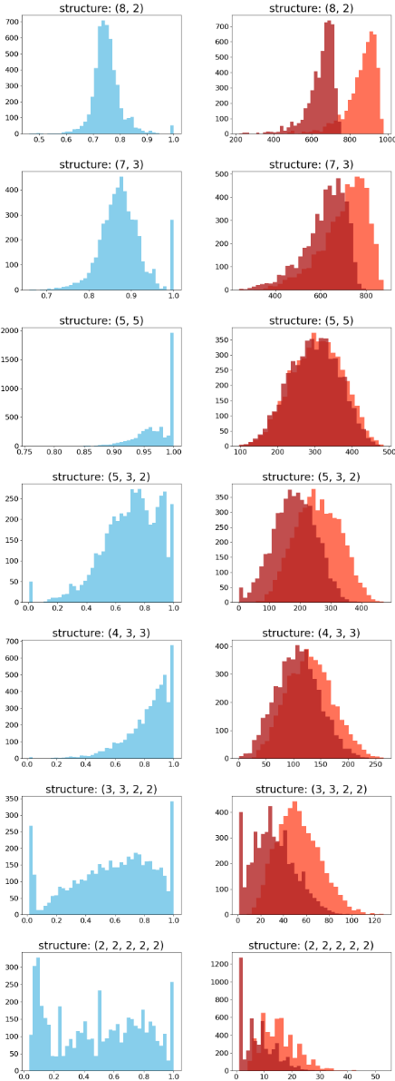
We first set the input dimension of the network as 7 and set the total number of neurons as 10. All the weights and biases follow the uniform distribution between -1 and 1. For the arrangements of neurons as (8, 2), (7, 3), (5, 5), (5, 3, 2), (4, 3, 3), (3, 3, 2, 2) and (2, 2, 2, 2, 2), we run the algorithm in Section 3 for 5000 times and get the number of linear regions, the number of activation regions as well as their ratio (i.e. #(linear regions)/#(activation regions) for each network generated in the experiment). The histograms for these three numbers are shown as Figure 3. We can see that Claim 1 holds in this case. Another observation is that the more similar the numbers of neurons in the layers are, the smaller the difference between the number of linear regions and that of activation regions is. Part 2 in Theorem 2.1 supports such phenomenon in the following sense. The gap 2n1 in (2.1) reflects the activation regions with constant values that are possible to be grouped together to form linear regions. In the proof of Theorem 2.1, when n1 = n2 = n, we can see that K(n1, n2) ≥ 3n 4 for n ≥ 4. So in this case, the larger n is, the smaller the gap 2n1 relative to K(n1, n2) (hence to E(N)) becomes. We also observe that for deep network structure such as (3, 3, 2, 2) and (2, 2, 2, 2, 2), the probability that there is only one linear region (i.e. the values of all the activation regions are constant) is quite high. The reason is that in this case it is easier for a neuron to drop out. For example, if the number of neurons in the k-th layer is nk, then if all the nk-1 weights towards a neuron in the k-th layer as well as the bias for that neuron are all non-positive, the neuron drops out, and this happens with probability 1 2nk-1+1 . In particular it is larger for smaller nk-1. Moreover, when there are only 2 neurons in a layer, it is also easier for these neurons to drop out simultaneously, resulting in only one linear region.
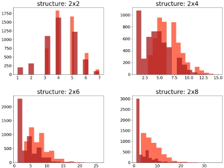
We also apply the algorithm on networks with input dimension 1, and compare the results from networks whose hidden layers are set as 2 × n and 2n × 1 for n = 2, 4, 6 and 8. One special property about such a pair of networks is that their total numbers of parameters are equal (both contain 4n weights and 2n + 1 biases). The number of linear regions of the networks of the form 2n × 1 is 2n + 1 with probability 1 according to (1.2), and the numbers for those of form 2 × n are shown as Figure 4. We can see clearly that in this case the shallow network (2n×1) still produces much more linear regions than the deep one (2×n). It seems that the probability of dropout mentioned in the previous paragraph is still an important factor for such gap.
4.2 Experiment on Two-Spiral Data
One may wonder whether the trend for randomly chosen parameters as in the previous subsection still exists for networks during training processes. Here we do an experiment for the two-spiral data which is widely used to train networks of small scale (e.g. [Sopena et al., 1999], [Hunter et al., 2012]). We follow the TensorFlow Playground [Google, 2016] to construct the two-spiral data as well as the input data which is of the form
except that we double the radii of the spirals. We take 500 points from each spiral and split the total data randomly into 900 training data and 100 test data. Observe that input dimension is 7 which is the same as Subsection 4.1. We train the networks whose hidden layers are arranged like those in 4.1, and calculate the numbers of linear regions for 30 networks in each accuracy range from 60%-69% to 90%-99%. The means and deviations of such numbers are shown as Table 1. There in the first column, we also include the means and deviations of the numbers of linear regions for the corresponding 5000 networks in 4.1. The "NC" there means excluding the case where the values are constant everywhere so that there is only one linear region.
We can see from Table 1 that the expectation of the numbers of linear regions for (8, 2), (7, 3) and (5, 5) with random parameters fits the estimation in (2.1). As for the expected number of linear regions during training, we can see slight decrease for the number for shallow networks (with hidden layers like (8, 2), (7, 3) and (5, 5)) and slight increase for deep networks (other networks structures), which makes the gap between the numbers for shallow and deep networks slightly smaller. However, such increase and decrease are trivial against the total number of linear regions and are far from enough to offset the gaps between different network structures. As a result, Claim 1 still holds here.
4.3 About Parallel Processing
Observe that in the algorithm in Section 3, for the Intersect, Add and Cut operation, each activation regions are handled individually and are independent of other regions. This provides room for optimization via parallel processing. In the parallel version of the algorithm, the whole pipeline is very similar to Figure 2, except that in the Intersect and Cut ◦Add operations, the activation regions are distributed to multiple machines and are processed there in parallel. However, due to the high complexity of the algorithm, even with parallel processing we still do not expect it to work for networks of industry scale. In fact, we have attempted to use a cluster of machines to run the algorithm and analyze networks trained on the MNIST dataset. From our experience, when the total number of neurons in the network is less than 20, the whole pipeline for a single network can barely be finished within a reasonable amount of time. This is still far from enough to handle the mainstream network structures which usually have a few hundred neurons (see [LeCun et al., 2010]).
5 Directions for Further Research
The results in this paper point out some directions which we think are worthy of further investigation as follows.
- Ideally, one can compare the expected of number of linear regions for all the network structures besides those in Theorem 1.1.
- Beyond Theorem 3.1 and Figure 3, there may be more interesting theoretical and practical results about the relationships between the number of linear regions and that of activation regions.
| Hidden layers Total mean & deviation | Accuracy range | Mean | Deviation |
|---|---|---|---|
| (8, 2) | 60%-69% | 645.24 | 63.23 |
| 647.69 & 72.24 | 70%-79% | 612.44 | 98.96 |
| 80%-89% | 635 | 74.13 | |
| 90%-99% | 563.8 | 166.05 | |
| (7, 3) | 60%-69% | 597.52 | 125.49 |
| 616.8046 & 94.02 | 70%-79% | 563.44 | 144.02 |
| 80%-89% | 634.52 | 111.47 | |
| 90%-99% | 547.16 | 111.86 | |
| (5, 5) | 60%-69% | 277.52 | 53.46 |
| 297.32 & 66.52 | 70%-79% | 299.68 | 71.20 |
| 80%-89% | 295.44 | 62.24 | |
| 90%-99% | 268.28 | 72.31 | |
| (5, 3, 2) | 60%-69% | 209.96 | 75.53 |
| 181.69 & 68.06 | 70%-79% | 205.28 | 71.76 |
| 80%-89% | 171.96 | 72.56 | |
| 90%-99% | 224.64 | 61.49 | |
| (4, 3, 3) | 60%-69% | 90.63 | 38.11 |
| 108.60 & 39.90 | 70%-79% | 114.4 | 26.64 |
| 80%-89% | 115.64 | 42.04 | |
| 90%-99% | 122.76 | 39.04 | |
| (3, 3, 2, 2) | 60%-69% | 41.36 | 19.44 |
| 31.35 & 18.60 | 70%-79% | 31.2 | 14.34 |
| (NC: 34.00 & 16.99) | 80%-89% | 37.68 | 21.15 |
| 90%-99% | 27.8 | 12.49 | |
| (2, 2, 2, 2, 2) | 60%-69% | 12.36 | 6.96 |
| 8.0 & 6.07 | 70%-79% | 11.4 | 3.38 |
| (NC: 10.39 & 5.20) | 80%-89% | 14.2 | 4.06 |
| 90%-99% | 14.6 | 5.97 |
@inproceedings{ijcai2022p492,
  title     = {Estimation and Comparison of Linear Regions for ReLU Networks},
  author    = {Wang, Yuan},
  booktitle = {Proceedings of the Thirty-First International Joint Conference on
               Artificial Intelligence, {IJCAI-22}},
  publisher = {International Joint Conferences on Artificial Intelligence Organization},
  editor    = {Luc De Raedt},
  pages     = {3544--3550},
  year      = {2022},
  month     = {7},
  note      = {Main Track},
  doi       = {10.24963/ijcai.2022/492},
  url       = {https://doi.org/10.24963/ijcai.2022/492},
}
TY - CPAPER TI - Estimation and Comparison of Linear Regions for ReLU Networks AU - Wang, Yuan T2 - Proceedings of the Thirty-First International Joint Conference on Artificial Intelligence, IJCAI-22 PB - International Joint Conferences on Artificial Intelligence Organization PY - 2022 SP - 3544 EP - 3550 DO - 10.24963/ijcai.2022/492 UR - https://doi.org/10.24963/ijcai.2022/492 ER -Copied
Machine-readable versions of this paper, for tools and AI agents:





