
Fine-Tuning Graph Neural Networks via Graph Topology Induced Optimal Transport
Proceedings of the Thirty-First International Joint Conference on Artificial Intelligence. Main Track. Pages 3730-3736.
https://doi.org/10.24963/ijcai.2022/518
Keywords
- Data Mining: Mining Graphs
- Machine Learning: Multi-task and Transfer Learning
- Machine Learning: Sequence and Graph Learning
Abstract
Recently, the pretrain-finetuning paradigm has attracted tons of attention in graph learning community due to its power of alleviating the lack of labels problem in many real-world applications. Current studies use existing techniques, such as weight constraint, representation constraint, which are derived from images or text data, to transfer the invariant knowledge from the pre-train stage to fine-tuning stage. However, these methods failed to preserve invariances from graph structure and Graph Neural Network (GNN) style models. In this paper, we present a novel optimal transport-based fine-tuning framework called GTOT-Tuning, namely, Graph Topology induced Optimal Transport fine-Tuning, for GNN style backbones. GTOT-Tuning is required to utilize the property of graph data to enhance the preservation of representation produced by fine-tuned networks. Toward this goal, we formulate graph local knowledge transfer as an Optimal Transport (OT) problem with a structural prior and construct the GTOT regularizer to constrain the fine-tuned model behaviors. By using the adjacency relationship amongst nodes, the GTOT regularizer achieves node-level optimal transport procedures and reduces redundant transport procedures, resulting in efficient knowledge transfer from the pre-trained models. We evaluate GTOT-Tuning on eight downstream tasks with various GNN backbones and demonstrate that it achieves state-of-the-art fine-tuning performance for GNNs.
- [Agrawal et al., 2014] Pulkit Agrawal, Ross Girshick, and Jitendra Malik. Analyzing the performance of multilayer neural networks for object recognition. In ECCV, 2014.
- [Bécigneul et al., 2020] Gary Bécigneul, Octavian-Eugen Ganea, and et al. Optimal transport graph neural networks. arXiv preprint arXiv:2006.04804, 2020.
- [Ben-David et al., 2007] Shai Ben-David, John Blitzer, Koby Crammer, Fernando Pereira, et al. Analysis of representations for domain adaptation. NeurIPS, 2007.
- [Bousquet and Elisseeff, 2002] Olivier Bousquet and André Elisseeff. Stability and generalization. JMLR, 2002.
- [Chen and Gan, 2020] Liqun Chen and Zhe et al. Gan. Graph optimal transport for cross-domain alignment. In ICML, pages 1542-1553, 2020.
- [Chen and Wang, 2021] Liqun Chen and Dong et al. Wang. Wasserstein contrastive representation distillation. In CVPR, pages 16296-16305, 2021.
- [Chen and Zhang, 2019] Liqun Chen and Yizhe et al. Zhang. Improving sequence-to-sequence learning via optimal transport. In ICLR, 2019.
- [Chen et al., 2019] Xinyang Chen, Sinan Wang, and et al. Catastrophic forgetting meets negative transfer: Batch spectral shrinkage for safe transfer learning. NeurIPS, 32:1908-1918, 2019.
- [Courty et al., 2016] Nicolas Courty, Rémi Flamary, Devis Tuia, and Alain Rakotomamonjy. Optimal transport for domain adaptation. TPAMI, 39(9):1853-1865, 2016.
- [Donahue and Jia, 2014] Jeff Donahue and Yangqing et al. Jia. Decaf: A deep convolutional activation feature for generic visual recognition. In ICML, pages 647-655, 2014.
- [Ganea et al., 2022] Octavian-Eugen Ganea, Xinyuan Huang, and et al. Independent SE(3)-equivariant models for end-to-end rigid protein docking. In ICLR, 2022.
- [He et al., 2019] Kaiming He, Ross Girshick, and Piotr Dollár. Rethinking imagenet pre-training. In ICCV, pages 4918-4927, 2019.
- [Hu et al., 2020] W Hu, B Liu, J Gomes, M Zitnik, P Liang, V Pande, and J Leskovec. Strategies for pre-training graph neural networks. In ICLR (ICLR), 2020.
- [Ji et al., 2022] Yuanfeng Ji, Lu Zhang, and et al. DrugOOD: Out-of-Distribution (OOD) Dataset Curator and Bench- mark for AI-aided Drug Discovery -A Focus on Affin- ity Prediction Problems with Noise Annotations. arXiv e-prints, page arXiv:2201.09637, January 2022.
- [Kou et al., 2020] Zhi Kou, Kaichao You, and et al. Stochas- tic normalization. NeurIPS, 33, 2020.
- [Li et al., 2018a] Qimai Li, Zhichao Han, and Xiao-Ming Wu. Deeper insights into graph convolutional networks for semi-supervised learning. In AAAI, 2018.
- [Li et al., 2018b] Xingjian Li, Haoyi Xiong, and et al. Delta: Deep learning transfer using feature map with attention for convolutional networks. In ICLR, 2018.
- [Li et al., 2020] Xuhong Li, Yves Grandvalet, Rémi Fla- mary, Nicolas Courty, and Dejing Dou. Represen- tation transfer by optimal transport. arXiv preprint arXiv:2007.06737, 2020.
- [Oquab et al., 2014] Maxime Oquab, Leon Bottou, Ivan Laptev, and Josef Sivic. Learning and transferring mid- level image representations using convolutional neural net- works. In CVPR, pages 1717-1724, 2014.
- [Peng et al., 2020] Zhen Peng, Wenbing Huang, and et al. Graph representation learning via graphical mutual infor- mation maximization. In The WebConf, 2020.
- [Peyré and Cuturi, 2019] Gabriel Peyré and Marco Cuturi. Computational optimal transport. Foundations and Trends in Machine Learning, 11 (5-6):355-602, 2019.
- [Rong et al., 2020] Yu Rong, Yatao Bian, and et al. Self- supervised graph transformer on large-scale molecular data. In NeurIPS, 2020.
- [Wu et al., 2018] Zhenqin Wu, Bharath Ramsundar, and et al. Moleculenet: a benchmark for molecular machine learning. Chemical science, 9(2):513-530, 2018.
- [Xu and et al., 2020] Renjun Xu and et al. Reliable weighted optimal transport for unsupervised domain adaptation. In CVPR, pages 4394-4403, 2020.
- [Xu and et al., 2021] Minghao Xu and et al. Self-supervised graph-level representation learning with local and global structure. ICML, 2021.
- [Xu et al., 2018] Keyulu Xu, Weihua Hu, Jure Leskovec, and Stefanie Jegelka. How powerful are graph neural net- works? In ICLR, 2018.
- [Xu et al., 2019] Hongteng Xu, Dixin Luo, and et al. Gromov-wasserstein learning for graph matching and node embedding. In ICML. PMLR, 2019.
- [Xuhong et al., 2018] LI Xuhong, Yves Grandvalet, and Franck Davoine. Explicit inductive bias for transfer learn- ing with convolutional networks. In ICML, 2018.
- [Yosinski et al., 2014] Jason Yosinski, Jeff Clune, and et al. How transferable are features in deep neural networks? NeurIPS, 27:3320-3328, 2014.
- [You et al., 2020] Yuning You, Tianlong Chen, Yongduo Sui, Ting Chen, Zhangyang Wang, and Yang Shen. Graph con- trastive learning with augmentations. NeurIPS, 2020.
- [Zhang et al., 2022] Jiying Zhang, Fuyang Li, Xi Xiao, Tingyang Xu, Yu Rong, Junzhou Huang, and Yatao Bian. Hypergraph convolutional networks via equivalency be- tween hypergraphs and undirected graphs. ICML TAG-ML Workshop, 2022.
References were extracted automatically from the PDF and may contain errors.
Full text extracted automatically from the PDF; figures, tables and equations may differ. The PDF is the version of record.
1 Introduction
Learning from limited number of training instances is a fundamental problem in many real-word applications. A popular approach to address this issue is fine-tuning a model that pretrains on a large dataset. In contrast to training from scratch, fine-tuning usually requires fewer labeled data, allows for faster training, and generally achieves better performance [Li et al., 2018b; He et al., 2019; Peng et al., 2020].
∗Correspondence to: Yatao Bian and Xi Xiao
1 Code: https://github.com/youjibiying/GTOT-Tuning.
Conventional fine-tuning approaches can be roughly divided into two categories: (i) weight constraint [Xuhong et al., 2018], i.e. directly constraining the distance of the weights between pretrained and finetuned models. Obviously, they would fail to utilize the topological information of graph data. (ii) representation constraint [Li et al., 2018b]. This type of approach constrains the distance of representations produced from pretrained and finetuned models, preserving the outputs or intermediate activations of finetuned networks. Therefore, both types of approaches fail to take good account of the topological information implied by the middle layer embeddings. However, it has been proven that GNNs explicitly look into the topological structure of the data by exploring the local and global semantics of the graph [Xu et al., 2018; Hu et al., 2020; Xu and et al., 2021; Peng et al., 2020; Zhang et al., 2022], which means that the implicit structure between the node embeddings is very significant. As a result, these fine-tuning methods, which cover only weights or layer activations and ignore the topological context of the input data, are no longer capable of obtaining comprehensive knowledge transfer.
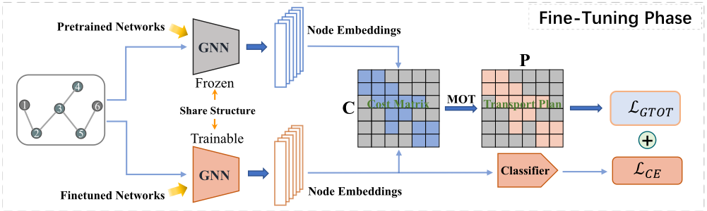
To preserve the local information of finetuned network from pretrained models, in this paper, we explore a principled representation regularization approach. i) Masked Optimal Transport (MOT) is formalized and used as a knowledge transfer procedure between pretrained and finetuned models. Compared with the Typical OT distance [Peyr´e and Cuturi, 2019], which considers all pair-wise distance between two domains [Courty et al., 2016], MOT allows for choosing the specific node pairs to sum in the final OT distance due to the introduced mask matrix. ii) The topological information of graphs is incorporated into the Masked Wasserstein distance (MWD) via setting the mask matrix as an adjacency matrix, leading to a GTOT distance within the node embedding space. The embedding distance between finetuned and pretrained models is minimized by penalizing the GTOT distance, preserving the local information of finetuned models from pretrained models. Finally, we propose a new finetuning framework: GTOT-Tuning as illustrated in Fig. 1.
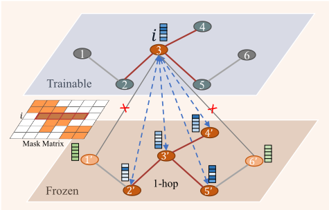
Using the adjacency relationship between nodes, the proposed GTOT regularizer achieves precise node-level optimal transport procedures and omits unnecessary transport procedures, resulting in efficient knowledge transfer from the pretrained models (Fig. 2). Moreover, thanks to the OT optimization that dynamically updates the transport map (weights to summing cosine dissimilarity) during training, the proposed regularizer is able to adaptively and implicitly adjust the distance between fine-tuned weights and pre-trained weights according to the downstream task. The experiments conducted on eight different datasets with various GNN backbones show that GTOT-Tuning achieves the best performance among all baselines, validating the effectiveness and generalization ability of our method.
Contributions: 1) We propose a masked OT problem as an extension of the classical Optimal Transport problem by introducing a mask matrix to constrain the transport procedures. Specially, we define Masked Wasserstein distance (MWD) for providing a flexible metric to compare two distributions. 2) We propose a fine-tuning framework called GTOT-Tuning tailored for GNNs, based on the proposed MWD. The core component of this framework, GTOT Regularizer, has the ability to utilize graph structure to preserve the local feature invariances between finetuned and pretrained models. To the best of our knowledge, it is the first fine-tuning method tailored for GNNs. 3) Empirically, we conduct extensive experiments on various benchmark datasets, and the results demonstrate a competitive performance of our method.
2 RelatedWork
Pretraining GNNs. Pre-training techniques have been shown to be effective for improving the generalization ability of GNN models. The existing methods for pre-training GNNs are mainly based on self-supervised paradigms. Some self-supervised tasks, e.g. context prediction [Hu et al., 2020; Rong et al., 2020], edge/attribute generation [Hu et al., 2020] and contrastive learning ([You et al., 2020; Xu and et al., 2021]), have been designed to obtain knowledge from unlabeled graphs. However, most of these methods only use the vanilla fine-tuning methods, i.e. the pretrained weights act as the initial weights for downstream tasks. It remains open to exploiting the optimal performance of the pre-trained GNN models. Our work is expected to utilize the graph structure to achieve better performance on the downstream tasks.
Fine-Tuning in Transfer Learning. Fine-tuning a pretrained model to downstream tasks is a popular paradigm in transfer learning (TL). [Donahue and Jia, 2014; Oquab et al., 2014] indicate that transferring features extracted by pre-trained AlexNet model to downstream tasks yields better performance than hand-crafted features. Further studies by [Yosinski et al., 2014; Agrawal et al., 2014] show that fine-tuning the pre-trained networks is more effective than fixed pre-trained representations. Recent research primarily focuses on how to better tap into the prior knowledge of pre-trained models from various perspectives. i) Weights: L2 SP [Xuhong et al., 2018] propose a L2 distance regularization that penalizes L2 distance between the fine-tuned weights and pre-trained weights. ii) Features: DELTA [Li et al., 2018b] constrains feature maps with the pre-trained activations selected by channel-wise attention. iii) Architecture: BSS [Chen et al., 2019] penalizes smaller singular values to suppress untransferable spectral components to prevent negative transfer. StochNorm [Kou et al., 2020] uses Stochastic Normalization to replace the classical batch normalization of pre-trained models. Despite the encouraging progress, it still lacks a fine-tuning method specifically for GNNs.
Optimal Transport. Optimal Transport is frequently used in many applications of deep learning, including domain adaption [Courty et al., 2016; Xu and et al., 2020], knowledge distillation [Chen and Wang, 2021], sequence-to-sequence learning [Chen and Zhang, 2019], graph matching [Xu et al., 2019], cross-domain alignment [Chen and Gan, 2020], rigid protein docking [Ganea et al., 2022], and GNN architecture design [B´ecigneul et al., 2020]. Some classical solutions to OT problem like Sinkhorn Algorithm can be found in [Peyr´e and Cuturi, 2019]. The work closely related to us may be [Li et al., 2020], which raises a fine-tuning method based on typical OT. The significant differences are that our approach is i) based on the proposed MOT, ii) tailored for GNNs, and iii) able to exploit the structural information of graphs.
3 Preliminaries
Notations. We define the inner product ⟨·, ·⟩ for matrices U,V ∈ Rm×n by ⟨U,V⟩ = tr(U⊤V) = ∑i,j UijVij. I ∈ Rn×n denotes the identity matrix, and 1n ∈ Rn represents the vector with ones in each component of size n. We use boldface letter x ∈ Rn to indicate an n-dimensional vector, where xi is the ith entry of x. Let G(V, E) be a graph with vertices V and edges E. We denote by A ∈ R|V|×|V| the adjacency matrix of G and ⊙ the Hadamard product. For convenience, we follow the terms of transfer learning and call the signal graph output from fine-tuned models (target networks) as target graph, and correspondingly, the output from pre-trained models (source networks) is called source graph. Note that these two graphs have the same adjacency matrix in fine-tuning setting.
Wasserstein Distance. Wasserstein distance (WD) [Peyr´e and Cuturi, 2019] is commonly used for matching two empirical distributions (e.g., two sets of node embeddings in a graph) [Courty et al., 2016]. The WD can be defined below.
Definition 1. Let α = ∑ni aiδxi and β = ∑mi biδy be two discrete distributions with δxi as the Dirac function concentrated at location x. Π(α, β) denotes all the joint distributions γ(x, y), with marginals α(x) and β(y). a ∈ Rn+ and b ∈ Rm+ are weight vectors satisfying ∑ni=1 ai = ∑mi=1 bi = 1. The definition of Wasserstein distance between the two discrete distributions α, β is:
where U(a, b) = {P ∈ Rn×m | P1m = a, P⊤1n = b} and Cij = c(xi, yj) is a cost scalar representing the distance between xi and yj . The P ∈ Rn×m is called as transport plan or transport map, and Pij represents the amount of mass to be moved from ai to bj. a, b are also known as marginal distributions of P.
The discrepancy between each pair of samples across the two domains can be measured by the optimal transport distance Dw(α, β). This seems to imply that Lw(a, b) is a natural choice as a representation distance between source graph and target graph for GNN fine-tuning. However, the local dependence exists between source and target graph, especially when the graph is large (see section 5). Therefore, it is not appropriate for WD to sum the distances of all node pairs. Inspired by this observation, we propose a masked optimal transport problem, as an extension of typical OT (section 4).
4 Masked Optimal Transport
Recall that in typical OT (definition 1), ai can be transported to any bj ∈ {bk}mk=1 with amount Pij . Here, we assume that the ai can only be transported to bj ∈ U where U ⊆ {bk}mk=1 is a subset. This constraint can be implemented by limiting the transport plan: Pij = 0 if bj /∈ U. Thus, the problem is formalized as follows by introducing the mask matrix.
Definition 2 (Masked Wasserstein Distance). Following the same notation of definition 1 and given a mask matrix M2 ∈ {0, 1}n×m where every row or column is not all zeros, the masked Wasserstein distance (MWD) is defined as
2 In this paper, Mij = 0 represents the ij-th element of the matrix being masked. Full Paper: https://arxiv.org/abs/2203.10453
Algorithm 1 Computing Masked Wasserstein Distance
Input: Cost matrix C, Mask matrix M ∈ {0, 1}n×m, Marginals a ∈ Rn+, b ∈ Rm+ , Iteration number K.
end for
where U(M, a, b) := {P ∈ Rn×m + | (M⊙P)1m = a, (M⊙ P)⊤1n = b, P ⊙ (1n×m - M) = 0n×m} and C ∈ Rn×m is a cost matrix.
From Eq. (3), the mask matrix M indicates that the elements of P need to be optimized, in other words, the costs need to be involved in the summation when calculating the inner product. Notably, different mask matrices M lead to different transport maps and obtain the OT distance associated with M. One can design M carefully to get a specific WD. Moreover, the defined MWD can recover WD by setting M = 1n×m and it is obvious that Lmw(M, a, b) ≥ Lw(a, b). This problem can obtain approximate solutions by adding an entropic regularization penalty, which is essential for deriving algorithms suitable for parallel iterations [Peyr´e and Cuturi, 2019].
Proposition 1. The solution to definition 2 with entropic regularization ϵH(M⊙P)3 is unique and has the form
where Kij = exp(-Cij/ϵ) and (u, v) ∈ Rn+ × Rm+ are two unknown scaling variables.
It is clear from the result that MWD is not equivalent to weighting the distance matrix C directly [Xu and et al., 2020], so the masked OT problem is nontrivial. We provide the proof in Appendix and the key to it is the observation that exp(M ⊙ X) = M ⊙ exp(X) + 1n×m -M, where X ∈ Rn×m is an arbitrary given matrix.
A conceptually simple method to compute the solution would be through the Sinkhorn Knopp iterations. However, as we know, the Sinkhorn algorithm suffers from numerical overflow when the regularization parameter ϵ is too small compared to the entries of the cost matrix C [Peyr´e and Cuturi, 2019]. This problem may be more severe when the sparsity of the mask matrix is large. Fortunately, this concern can be somewhat alleviated by performing computations in the log domain. Therefore, for numerical stability and speed, we propose the Log-domain masked Sinkhorn algorithm (the derivation can be seen in Appendix). Algorithm 1 provides the whole process.
3 Namely, min P∈U(M,a,b) ⟨M ⊙ P, C⟩-ϵH(M⊙P), where H(·) is
Entropy function. Assume that 0 log 0 = 0 to ensure that H(M⊙P) is well defined.
5 Fine-Tuning GNNs viaMasked OT Distance
In our proposed framework, we use Masked Optimal Transport (MOT) for GNNs fine-tuning, where a transport plan P ∈ Rn×m is learned to optimize the knowledge transfer between pretrained and fine-tuned models. There are several distinctive characteristics of MOT that make it an ideal tool for fine-tuning GNNs. (i) Self normalization: All the elements of P sum to 1. (ii) Sparsity: The introduced mask matrix can effectively limit the sparsity of the transport map, leading to a more interpretable and robust representation regularizer for fine-tuning ( See Fig. 12 in Appendix.). (iii) Efficiency: Our solution can be easily obtained by Algorithm 1 that only requires matrix-vector products, therefore is readily applicable to GNNs. (iv) Flexibility: The Masked matrix can assign exclusive transport plans for specific transport tasks and reduce the unnecessary optimal transport procedure.
5.1 GTOT Regularizer
Given the node embeddings {xSi }|V| i=1 and {xTi }|V| i=1 extracted from pre-trained GNN and fine-tuned GNN message passing period, respectively, we calculate the cosine dissimilarity Cij = 12 (1 - cos(xSi , xTj )) as the cost matrix of MWD. Indeed, cosine dissimilarity is a popular choice that used in many OT application [Chen and Gan, 2020; Xu and et al., 2020]. Intuitively, in most cases, the more (geodesic) distant two vertices in a graph are, the less similar their features are. This implies that when the MWD is used for finetuning, the adjacency of the graph should be taken into account, rather than summing all pairwise distances of the cost matrix. Therefore, we set the mask matrix as the adjacency matrix A (with self-loop) here, based on the assumption of 1-hop dependence, i.e., the vertices in the target graph are assumed to be related only to the vertices within 1-hop of the corresponding vertices in the source graph (Fig. 2). This assumption is reasonable because the neighboring node embeddings extracted through the (pretrained) GNN are somewhat similar [Li et al., 2018a], which also reveals that considering only the node-to-node distance but without the neighbors is sub-optimal. We call this MOT with graph topology as Graph Topology induced Optimal Transport (GTOT). With marginal distributions being uniform, the GTOT regularizer is formally defined as
where q is defined as uniform distribution 1|V|/|V|. Noted that the inner product in Eq. (5) can be rewritten as ∑i ∑j∈N(i) ⋃{i} PijCij, where N(i) denotes the set of neighbors of node i. Moreover, our method has the potential to use sparse matrix acceleration when the adjacency matrix is sparse. Our method is easy to extend to i) the weighted graph by element-wise multiplying the edge-weighted matrix W with cost matrix, i.e. ⟨A⊙P,W⊙C⟩ or ii) the k-hop dependence assumption by replacing A with Ak or g(A), where g is a polynomial function. Similarly, using MOT we can define the MGWD-based Regularizer for regularizing the representations on edge-level (see appendix).
5.2 GTOT-Tuning Framework
Unlike the OT representation regularizer proposed by [Li et al., 2020] which calculates the Wasserstein distance between mini-batch samples of training data, GTOT regularizer in our framework focus on the single sample, that is, the GTOT distance between the node embeddings of one source graph and the corresponding target graph. Considering the GTOT distance between nodes allows for knowledge transfer at the node level. This makes the fine-tuned model able to output representations that are more appropriate for the downstream task, i.e., node representations that are as identical as possible to these output from the pre-trained model, but with specific differences in the graph-level representations.
Overall Objective. Given N training samples {(G1, y1), · · · , (GN, yN)}, the overall objective of GTOTTuning is to minimize the following loss:
where l(f, Gi, yi) := ϕ(f(Gi), yi)+λLmw(A(i) , q(i) , q(i) ), f denotes a given GNN backbone, λ is a hyper-parameter for balancing the regularization with the main loss function, and ϕ(·) is Cross Entropy loss function.
| Datasets | BBBP | Tox21 | Toxcast | SIDER | ClinTox | MUV | HIV | BACE | Average |
|---|---|---|---|---|---|---|---|---|---|
| Methods | GIN (contexpred) | ||||||||
| Fine-Tuning (baseline) | 68.0±2.0 | 75.7±0.7 | 63.9±0.6 | 60.9±0.6 | 65.9±3.8 | 75.8±1.7 | 77.3±1.0 | 79.6±1.2 | 70.85 |
| L2 SP [Xuhong et al., 2018] DELTA[Li et al., 2018b] Feature(DELTA w/o ATT) | 68.2±0.7 | 73.6±0.8 | 62.4±0.3 | 61.1±0.7 | 68.1±3.7 | 76.7±0.9 | 75.7±1.5 | 82.2±2.4 | 70.25 |
| 67.8±0.8 | 75.2±0.5 | 63.3±0.5 | 62.2±0.4 | 73.4±3.0 | 80.2±1.1 | 77.5±0.9 | 81.8±1.1 | 72.68 | |
| 61.4±0.8 | 71.1±0.1 | 61.5±0.2 | 62.4±0.3 | 64.0±3.4 | 78.4±1.1 | 74.0±0.5 | 76.3±1.1 | 68.64 | |
| BSS[Chen et al., 2019] | 68.1±1.4 | 75.9±0.8 | 63.9±0.4 | 60.9±0.8 | 70.9±5.1 | 78.0±2.0 | 77.6±0.8 | 82.4±1.8 | 72.21 |
| StochNorm [Kou et al., 2020] | 69.3±1.6 | 74.9±0.6 | 63.4±0.5 | 61.0±1.1 | 65.5±4.2 | 76.0±1.6 | 77.6±0.8 | 80.5±2.7 | 71.03 |
| GTOT-Tuning (Ours) | 70.0±2.3 | 75.6±0.7 | 64.0±0.3 | 63.5±0.6 | 72.0±5.4 | 80.0±1.8 | 78.2±0.7 | 83.4±1.9 | 73.34 |
| Methods | GIN (supervised contexpred) | ||||||||
| Fine-Tuning (baseline) | 68.7±1.3 | 78.1±0.6 | 65.7±0.6 | 62.7±0.8 | 72.6±1.5 | 81.3±2.1 | 79.9±0.7 | 84.5±0.7 | 74.19 |
| L2 SP [Xuhong et al., 2018] | 68.5±1.0 | 78.7±0.3 | 65.7±0.4 | 63.8±0.3 | 71.8±1.6 | 85.0±1.1 | 77.5±0.9 | 84.5±0.9 | 74.44 |
| DELTA[Li et al., 2018b] | 68.4±1.2 | 77.9±0.2 | 65.6±0.2 | 62.9±0.8 | 72.7±1.9 | 85.9±1.3 | 75.6±0.4 | 79.0±1.1 | 73.50 |
| Feature(DELTA w/o ATT) | 68.6±0.9 | 77.9±0.2 | 65.7±0.2 | 63.0±0.6 | 72.7±1.5 | 85.6±1.0 | 75.7±0.3 | 78.4±0.7 | 73.45 |
| BSS[Chen et al., 2019] | 70.0±1.0 | 78.3±0.4 | 65.8±0.3 | 62.8±0.6 | 73.7±1.3 | 78.6±2.1 | 79.9±1.4 | 84.2±1.0 | 74.16 |
| StochNorm [Kou et al., 2020] | 69.8±0.9 | 78.4±0.3 | 66.1±0.4 | 62.2±0.7 | 73.2±2.1 | 82.5±2.6 | 80.2±0.7 | 84.2±2.3 | 74.58 |
| GTOT-Tuning (Ours) | 71.5±0.8 | 78.6±0.3 | 66.6±0.4 | 63.3±0.6 | 77.9±3.2 | 85.0±0.9 | 81.1±0.5 | 85.3±1.5 | 76.16 |
6 Theoretical Analysis
We provide some theoretical analysis for GTOT-Tuning.
Algorithm Stability and Generalization Bound. We analyze the generalization bound of GTOT-Tuning and expect to find the key factors that affect its generalization ability. We first give the uniform stability below.
Lemma 1 (Uniform stability for GTOT-Tuning). Let S := {z1 = (G1, y1), z2 = (G2, y2), · · · , zi-1 = (Gi-1, yi-1), zi = (Gi, yi), zi+1 = (Gi+1, yi+1), · · · , zN = (GN, yN)} be a training set with N graphs, Si := {G1,G2, ...,Gi-1,G′i ,Gi+1, ...,GN} be the training set where graph i has been replaced. Assume that the number of vertices |VGj | ≤ B for all j and 0 ≤ ϕ(fS, z) ≤ M, then
where λ is the hyper-parameter used in Eq. (6).
Based on Lemma 1 and following the conclusion of [Bousquet and Elisseeff, 2002], the generalization error bound of GTOT-Tuning is obtained as follows.
Proposition 2. Assume that a GNN with GTOT regularization satisfies 0 ≤ l(fS, z) ≤ Q. For any δ ∈ (0, 1), the following bound holds with probability at least 1-δ over the random draw of the sample S,
where R(fS) denotes the generalization error and Rm(fS) represents empirical error. Proof is deferred to Appendix.
This result shows that the generalization bound of GNN with GTOT regularizer is affected by the maximum number of vertices (B) in the training dataset.
7 Empirical Studies
We conduct experiments on graph classification tasks to evaluate our method.
7.1 Comparison of Various Fine-Tuning Strategies
We compare our method with other Fine-Tuning Strategies as follows.
Settings. We reuse two pretrained models released by [Hu et al., 2020] as backbones: GIN (contextpred) [Xu et al., 2018], which is only pretrained via self-supervised task Context Prediction, and GIN (supervised contextpred), an architecture that is pretrained by Context Prediction + Graph Level multi-task supervised strategy. Both networks are pre-trained on the Chemistry dataset (with 2 million molecules). In addition, eight binary classification datasets in MoleculeNet [Wu et al., 2018] serve as downstream tasks for evaluating the finetuning strategies, where the scaffold split scheme is used for dataset split. More details can be found in Appendix.
Baselines. Since we have not found related works about fine-tuning GNNs, we extend several typical baselines tailored for Convolutional networks to GNNs, including L2 SP, DELTA, BSS, SotchNorm.
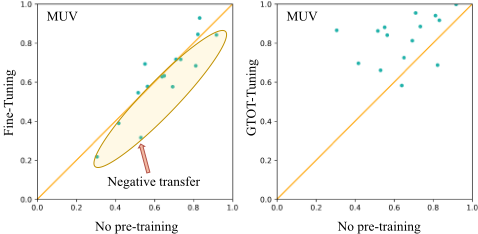
Results. The results with different fine-tuning strategies are shown in Table 1. Observation (1): GTOT-Tuning gains a competitive performance on different datasets and outperforms other methods on average. Observation (2): Weights regularization (L2 SP) can't obtain improvement on pure self-supervised tasks. This implies L2 SP may require the pretrained task to be similar to the downstream task. Fortunately, our method can consistently boost the performance of both supervised and self-supervised pretrained models. Observation (3): The performance of the Euclidean distance regularization (Features(DELTA w/o ATT)) is worse than vanilla fine-tuning, indicating that directly using the node representation regularization may cause negative transfer.
7.2 Ablation Studies
Effects of the Mask Matrix. We conduct the experiments on GNNs fine-tuning with GTOT regularizer to verify the efficiency of the introduced adjacency matrix. The results shown in Table 2 suggest that when using adjacency matrix as mask matrix, the performance on most downstream tasks will be better than using classic WD directly. Besides, the competitive performance when the mask matrix is identity also implies that we can select possible pre-designed mask matrices, such as polynomials of A, for specific downstream tasks. This also indicates that our MOT can be flexibly used for fine-tuning. (MWD(A) is GTOT distance.)
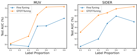
Effects of Different Proportion of LabeledData. We also investigate the performance of the proposed method with different proportions of labeled data on MUV and SIDER datasets. As illustrated in Fig. 3, MWD outperforms the baseline (vanilla Fine-Tuning) given different amounts of labeled data consistently, indicating the generalization of our method.
| Methods | BBBP | Tox21 | Toxcast | SIDER |
|---|---|---|---|---|
| # A distance | 1.57 | 1.56 | 1.56 | 1.41 |
| w/o MWD w/ MWD(1n×n) w/ MWD(A) w/ MWD(I) | 68.7±3.4 | 75.9±0.5 | 63.1±0.6 | 60.2±0.9 |
| 66.2±3.3 | 75.3±0.9 | 63.6±0.6 | 62.7±0.7 | |
| 69.6±2.6 | 75.7±0.5 | 63.8±0.4 | 63.5±0.6 | |
| 68.6±3.5 | 75.4±0.7 | 64.1±0.3 | 63.7±0.5 | |
| Methods | ClinTox | MUV | HIV | BACE |
| # A distance | 1.41 | 1.19 | 1.65 | 1.65 |
| w/o MWD w/ w/ | 69.5±5.0 | 69.5±1.3 | 78.2±1.2 | 82.5±1.7 |
| MWD(1n×n) | 69.5±5.0 | 74.3±1.3 | 78.2±0.8 | 83.7±1.9 |
| MWD(A) | 70.9±5.8 | 80.7±0.6 | 78.5±1.5 | 83.1±1.9 |
| w/ MWD(I) | 69.7±4.0 | 80.2±0.9 | 78.3±1.3 | 82.6±2.5 |
7.3 Why GTOT-TuningWorks
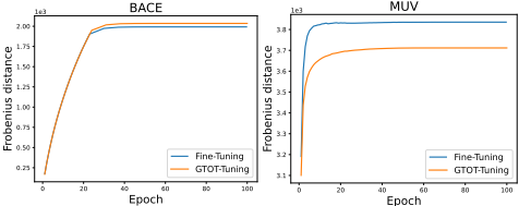
Adaptive Adjustment of Model Weights to Downstream Tasks. The A-distance [Ben-David et al., 2007], dA(DS , DT ) = 2(1 - 2ξ(h)) is adopted to measure the discrepancy between the pretrained and finetuned domains, i.e. the domain gap between pre-trained data DS and fine-tuned data DT . ξ(h) is the error of a linear SVM classifier h discriminating the two domains [Xu and et al., 2020]. We calculate the dA with representations extracted by GIN (contextpred) as input and show the results in Table 2. From Fig. 4, it can be observed that GTOT-Tuning constrains the weights distance between fine-tuned and pre-trained model when domain gap is relatively small (MUV). Conversely, when the domain gap is large (BACE), our method does not necessarily increase the distance between weights, but rather increases the distance between weights. This reveals that GOT-Tuning can adaptively and implicitly adjust the distance between fine-tuned weights and pre-trained weights according to the downstream task, yielding powerful fine-tuned models.
Mitigating Negative Transfer under Multi-task. Fig. 5 shows that GTOT-Tuning boosts the performance of most tasks on multi-task datasets, demonstrating the ability of our method in mitigating negative transfer.
8 Discussions and FutureWork
Despite the good results, there are some aspects which worth further explorations: i) The MOT-based methods require relatively high computational cost, which calls for designing a more efficient algorithm to solve it. ii) MWD has the potential to perform even better when used in conjunction with MGWD. iii) The proposed method can be potentially extended for more challenging settings that needs advanced knowledge transfer techniques, such as the graph out of distribution learning [Ji et al., 2022].
Acknowledgments
This work was supported in part by the National Natural Science Foundation of China (61972219), the Research and Development Program of Shenzhen (JCYJ20190813174403598, SGDX20190918101201696), the National Key Research and Development Program of China (2018YFB1800601), and the Overseas Research Cooperation Fund of Tsinghua Shenzhen International Graduate School (HW2021013). Besides, the authors would like to thank Ximei Wang, Guoji Fu and Guanzi Chen for their sincere and selfless help.
@inproceedings{ijcai2022p518,
  title     = {Fine-Tuning Graph Neural Networks via Graph Topology Induced Optimal Transport},
  author    = {Zhang, Jiying and Xiao, Xi and Huang, Long-Kai and Rong, Yu and Bian, Yatao},
  booktitle = {Proceedings of the Thirty-First International Joint Conference on
               Artificial Intelligence, {IJCAI-22}},
  publisher = {International Joint Conferences on Artificial Intelligence Organization},
  editor    = {Luc De Raedt},
  pages     = {3730--3736},
  year      = {2022},
  month     = {7},
  note      = {Main Track},
  doi       = {10.24963/ijcai.2022/518},
  url       = {https://doi.org/10.24963/ijcai.2022/518},
}
TY - CPAPER TI - Fine-Tuning Graph Neural Networks via Graph Topology Induced Optimal Transport AU - Zhang, Jiying AU - Xiao, Xi AU - Huang, Long-Kai AU - Rong, Yu AU - Bian, Yatao T2 - Proceedings of the Thirty-First International Joint Conference on Artificial Intelligence, IJCAI-22 PB - International Joint Conferences on Artificial Intelligence Organization PY - 2022 SP - 3730 EP - 3736 DO - 10.24963/ijcai.2022/518 UR - https://doi.org/10.24963/ijcai.2022/518 ER -Copied
Machine-readable versions of this paper, for tools and AI agents:





