
Temporality Spatialization: A Scalable and Faithful Time-Travelling Visualization for Deep Classifier Training
Proceedings of the Thirty-First International Joint Conference on Artificial Intelligence. Main Track. Pages 4022-4028.
https://doi.org/10.24963/ijcai.2022/558
Keywords
- AI Ethics, Trust, Fairness: Explainability and Interpretability
- Multidisciplinary Topics and Applications: Software Engineering
Abstract
Time-travelling visualization answers how the predictions of a deep classifier are formed during the training. It visualizes in two or three dimensional space how the classification boundaries and sample embeddings are evolved during training.
In this work, we propose TimeVis, a novel time-travelling visualization solution for deep classifiers. Comparing to the state-of-the-art solution DeepVisualInsight (DVI), TimeVis can significantly (1) reduce visualization errors for rendering samples’ travel across different training epochs, and (2) improve the visualization efficiency. To this end, we design a technique called temporality spatialization, which unifies the spatial relation (e.g., neighbouring samples in single epoch) and temporal relation (e.g., one identical sample in neighbouring training epochs) into one high-dimensional topological complex. Such spatio-temporal complex can be used to efficiently train one visualization model to accurately project and inverse-project any high and low dimensional data across epochs. Our extensive experiment shows that, in comparison to DVI, TimeVis not only is more accurate to preserve the visualized time-travelling semantics, but 15X faster in visualization efficiency, achieving a new state-of-the-art in time-travelling visualization.
- [Adebayo et al., 2018] Julius Adebayo, Justin Gilmer, Michael Muelly, Ian Goodfellow, Moritz Hardt, and Been Kim. Sanity checks for saliency maps. arXiv preprint arXiv:1810.03292, 2018.
- [Alsallakh et al., 2021] Bilal Alsallakh, Narine Kokhlikyan, Vivek Miglani, Shubham Muttepawar, Edward Wang, Sara Zhang, David Adkins, and Orion Reblitz-Richardson. De- bugging the internals of convolutional networks. In eX- plainable AI approaches for debugging and diagnosis., 2021.
- [Chattopadhyay et al., 2019] Aditya Chattopadhyay, Piyushi Manupriya, Anirban Sarkar, and Vineeth N Balasubrama- nian. Neural network attributions: A causal perspective. In International Conference on Machine Learning, pages 981-990. PMLR, 2019.
- [Chazal et al., 2014] Frédéric Chazal, Vin De Silva, and Steve Oudot. Persistence stability for geometric com- plexes. Geometriae Dedicata, 173(1):193-214, 2014.
- [Chazal et al., 2015] Frederic Chazal, Brittany Fasy, Fab- rizio Lecci, Bertrand Michel, Alessandro Rinaldo, and Larry Wasserman. Subsampling methods for persistent ho- mology. In Francis Bach and David Blei, editors, ICML, volume 37 of Proceedings of Machine Learning Research, pages 2143-2151, Lille, France, 07-09 Jul 2015. PMLR.
- [Chazal et al., 2016] Frédéric Chazal, Vin De Silva, Marc Glisse, and Steve Oudot. The structure and stability of persistence modules. Springer, 2016.
- [Facco et al., 2017] Elena Facco, Maria d'Errico, Alex Ro- driguez, and Alessandro Laio. Estimating the intrinsic di- mension of datasets by a minimal neighborhood informa- tion. Scientific reports, 7(1):1-8, 2017.
- [Farahani and Hekmatfar, 2009] Reza Zanjirani Farahani and Masoud Hekmatfar. Facility location: concepts, models, algorithms and case studies. Springer Science & Business Media, 2009.
- [Gonzalez, 1985] Teofilo F Gonzalez. Clustering to mini- mize the maximum intercluster distance. Theoretical com- puter science, 38:293-306, 1985.
- [Graving and Couzin, 2020] Jacob M Graving and Iain D Couzin. Vae-sne: a deep generative model for simulta- neous dimensionality reduction and clustering. BioRxiv, 2020.
- [Lin et al., 2017] Yun Lin, Jun Sun, Yinxing Xue, Yang Liu, and Jinsong Dong. Feedback-based debugging. In 2017 IEEE/ACM 39th International Conference on Software Engineering (ICSE), pages 393-403. IEEE, 2017.
- [Mallick et al., 2019] Koushik Mallick, Sanghamitra Bandy- opadhyay, Subhasis Chakraborty, Rounaq Choudhuri, and Sayan Bose. Topo2vec: A novel node embedding gen- eration based on network topology for link prediction. IEEE Transactions on Computational Social Systems, 6(6):1306-1317, 2019.
- [McInnes et al., 2018] Leland McInnes, John Healy, and James Melville. Umap: Uniform manifold approximation and projection for dimension reduction. arXiv preprint arXiv:1802.03426, 2018.
- [Moor et al., 2020] Michael Moor, Max Horn, Bastian Rieck, and Karsten Borgwardt. Topological autoencoders. In International conference on machine learning, pages 7045-7054. PMLR, 2020.
- [Sainburg et al., 2021] Tim Sainburg, Leland McInnes, and Timothy Q. Gentner. Parametric UMAP Embeddings for Representation and Semisupervised Learning. Neural Computation, 33(11):2881-2907, 10 2021.
- [Sener and Savarese, 2017] Ozan Sener and Silvio Savarese. Active learning for convolutional neural networks: A core- set approach. arXiv preprint arXiv:1708.00489, 2017.
- [Sundararajan et al., 2017] Mukund Sundararajan, Ankur Taly, and Qiqi Yan. Axiomatic attribution for deep net- works. In International Conference on Machine Learning, pages 3319-3328. PMLR, 2017.
- [Wang et al., 2019] Haijun Wang, Yun Lin, Zijiang Yang, Jun Sun, Yang Liu, Jin Song Dong, Qinghua Zheng, and Ting Liu. Explaining regressions via alignment slicing and mending. IEEE Transactions on Software Engineering, 2019.
- [Xiao et al., 2021] Yan Xiao, Ivan Beschastnikh, David S Rosenblum, Changsheng Sun, Sebastian Elbaum, Yun Lin, and Jin Song Dong. Self-checking deep neural networks in deployment. In 2021 IEEE/ACM 43rd International Con- ference on Software Engineering (ICSE), pages 372-384. IEEE, 2021.
- [Yang et al., 2022a] Xianglin Yang, Yun Lin, Ruofan Liu, and Jin Song Dong. Appendix. https://sites.google.com/ view/timevis/home, 2022. Accessed: 2022-01-15. Link
- [Yang et al., 2022b] Xianglin Yang, Yun Lin, Ruofan Liu, and Jin Song Dong. Website of timevis. https://sites. google.com/view/timevis/home, 2022. Accessed: 2022- 01-15. Link
- [Yang et al., 2022c] Xianglin Yang, Yun Lin, Ruofan Liu, Zhenfeng He, Chao Wang, Jin Song Dong, and Hong Mei. Deepvisualinsight: Time-travelling visualization for spatio-temporal causality of deep classification training. In The Thirty-Sixth AAAI Conference on Artificial Intel- ligence (AAAI), 2022.
- [Zeiler and Fergus, 2014] Matthew D Zeiler and Rob Fergus. Visualizing and understanding convolutional networks. In European conference on computer vision, pages 818-833. Springer, 2014.
References were extracted automatically from the PDF and may contain errors.
Full text extracted automatically from the PDF; figures, tables and equations may differ. The PDF is the version of record.
1 Introduction
Time-travelling visualization, solution to address how the deep model predictions are formed during the training, are emerging as a new branch of explainable AI [Yang et al., 2022c]. Such visualization demonstrates how the highdimensional classification landscape is learned during training, which can facilitate training-based causal inference on embedding generation [Mallick et al., 2019] and active learning algorithms [Sener and Savarese, 2017].
Any time-travelling visualization solutions for deep classifiers are required to fulfill three spatial properties and one temporal property so as to faithfully reflect the dynamics of high-dimensional classification landscape [Yang et al.,
∗Corresponding author
2022c]. Briefly, given a set of high-dimensional representations trained in epoch et, the three spatial properties are:
- Neighbour preserving property: The neighbours of any high-dimensional representation should be preserved after being projected into a visible low-dimensional space.
- Boundary distance preserving property: The relative distance from any high-dimensional representation to its closest classification boundary is preserved after being projected to a visible low-dimensional space.
- Inverse-projection preserving property: After projecting a high-dimensional representation x into low-dimensional space as y, we shall inverse-project x back to the highdimensional space as x′ such that x and x′ are similar.
Besides, the one temporal property requires:
- Temporal preserving property (continuity): If the neighbours of a high-dimensional representation xt+k (from epoch t + k) do not change much from its correspondence xt (from epoch t), then their low-dimensional projections yt+k and yt shall be close.
These properties ensure that the "animation" of a model's training process can be "played" reflectively (thanks to the spatial properties) and smoothly (thanks to the temporal property) in a visible low-dimensional space.
DeepVisualInsight (DVI), as a state-of-the-art, is further crystallized for fulfilling these properties [Yang et al., 2022c]. Technically, DVI trains visualization models as auto-encoders on several loss functions enforcing the properties. However, the solution has its limit on the visualization scalability and the faithfulness on the travelling semantics of samples across different epochs.
Problem 1: Visualization Scalability. Given that the classification landscape differs one epoch from another, the timetravelling visualization is generally a record-and-replay technique to record and visualize the partially-trained classifier in each epoch. DVI trains one visualization model on each time step. Hence, the visualization training process can be prohibitively costly, especially when the number of training epochs is large. Experiments report that training one visualization model at a normal GPU-workstation takes about 15 minutes [Yang et al., 2022c], which indicates that training the visualization models for 100 epochs takes around 24 hours. Even worse, in order to satisfy the temporal property, training the visualization models for the classifier at epoch et requires the availability of the visualization model at epoch et-1, which limits its paralleling potential.
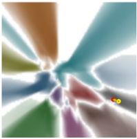
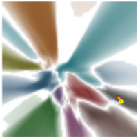
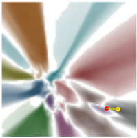
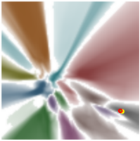
(d) epoch 100 (unexpected creation of a green territory)
Figure 1: The erroneous visualization perturbation of DVI while the classification semantics remain the same among the epochs: Each color represents a class, while the white region between the territories represents the classification boundary. Given a sample (i.e., a point), its color represents its label, and its background color represents its prediction. For example, being located in a territory of "bird" (green territory) means a sample is predicted as a bird. We show the erroneous fluctuation trajectory of a static sample. The point with yellow edge indicates the location of current epoch and that of red edge indicates its location of previous epoch.
Problem 2: Faithfulness of Travelling Semantics (Visualization Error). When we project the learned representations of a sample X = {x1 , x2 , . . . , xw } (xi indicates the sample representation at i-th epoch) to low-dimensional space in chronological order, their projections Y = {y1 , y2 , . . . , yw } form a travelling trajectory. When we observe the movement of yi to yi+1 on the two-dimensional canvas, it can be caused by (1) the actual movement from xi to xi+1 in the high-dimensional space and (2) the visualization perturbation or errors. We call the movement caused by the latter as the unfaithful movement of a sample. The visualization model is trained as V = ⟨ϕ, ψ⟩ where ϕ projects high-dimensional points to low-dimensional space and ψ inverse-projects lowdimensional points back to high-dimensional space. DVI trains the visualization model V = ⟨ϕ, ψ⟩ at epoch i + 1 by retraining from the visualization model at epoch i. The randomness-inducing retraining process can inevitably incur unintentional fluctuation to visualize the classification landscape. In addition, the temporal loss designed in DVI can freeze the minority of dynamic samples while the majority samples do not move in the high-dimensional space. As a result, the visualized travelling semantics cannot well faithfully reflect the dynamics in high-dimensional space.
In this work, we propose TimeVis to uniformly address the above problems by a technique called temporality spatialization. In comparison to DVI which trains a visualization model for each partially trained classifier, we train a visualization model to capture the representation embeddings of all the classifiers. Specifically, our approach "spatializes" the temporal relations of a sample and its correspondences in other epochs. In TimeVis, we regard every representation has both spatial neighbours and temporal neighbours. Technically, we (1) collect all appeared representation during the training, (2) construct a spatio-temporal complex to capture both spatial and temporal relation of the representations in the same highdimensional space, and (3) learn the dimensional projection and inverse-projection based on such complex. To further improve the visualization scalability, we propose a complexreduction technique for the spatio-temporal complex, which can successfully compress the size of the complex without compromising much visualization accuracy.
Our experiments on a variety of datasets show that, in comparison to DVI, TimeVis can (1) significantly improve the training scalability (15X faster), (2) largely improve travelling faithfulness, and (3) achieve comparable performance on the other spatial properties.
In summary, this work makes the following contributions:
- We identify two critical problems limiting the practical applicability of the emerging time-travelling visualization.
- We propose temporality spatialization to significantly improve the visualization scalability and visualization faithfulness of travelling semantics, achieving a new state-ofthe-art in time-travelling visualization.
- We build a tool TimeVis based on our technique to support its practical use, which is publicly available at [Yang et al., 2022b] and https://github.com/xianglinyang/TimeVis.
2 Motivation
Figure 1 shows the time-travelling visualization results of DVI at late training stage when training ResNet18 on the CIFAR10 dataset. At late stage, the semantics of the classifier converge. Generally, the loss, the training accuracy, and the testing accuracy do not change. Individually, the representations of almost all the training samples preserve their k nearest neighbours in those epochs.
However, DVI has two visualization errors which can cloud the understanding of the classification landscape. First, a green territory (i.e., the bird class) is created in the middle, locating near to the red territory (i.e., the cat class) from epoch 99 to epoch 100. However, the bird samples falling in this new green territory are no closer to the cat-image samples in the representation space. Second, we further observe some erroneous fluctuation of samples on the canvas. The sample moves back-and-forth during the four epochs as shown in Figure 1. On the contrary, both its representation and neighbours remain the same across the epochs in the high-dimensional space. The noisy visualization perturbation can misguide the user to doubt the training stableness, and misunderstand what exactly happen in the high-dimensional space. Due to space limit, we also show a "frozen" sample on the canvas by DVI on [Yang et al., 2022b], where the sample is very dynamic in the high-dimensional space.
3 ProblemDefinition
Given a dataset D = {s1, s2, ..., sn} in d dimensional space (n is the dataset size), a set of classes C = {c1, c2, ..., cm} (m is the number of class size), we have a sequence of w deep classifiers f 1 (·), f 2 (·), . . . , f w (·) taken in chronological order, where each f t : Rd → Rm is a learned classifier at the training epoch et. We assume that each deep classifier f t (·) can be decomposed into a feature function gt : Rd → Rr and a prediction function ht : Rr → Rm (i.e., f t = ht ◦ gt ) with r being the dimension of the representation space. Thus, we can derive a set of sample representations Xt = {xt1 , xt2 , . . . , xtn } for each epoch t, where xti = gt (si) ∈ Rr . Note that we use superscript and subscript to denote different time steps and different samples respectively. The learned representations of a sample si in different time steps are denoted as Xi = {x1i , x2i , . . . , xwi }.
We aim for one visualization model V = ⟨ϕ, ψ⟩ where ϕ : Rr → Rl and ψ : Rl → Rr (l ∈ {2, 3} is the dimension of the visible low-dimensional space). Given a visualization solution V = ⟨ϕ, ψ⟩, we (1) visualize each representation xti as yt i = ϕ(xti ) in a visible low-dimensional space; and (2) paint any point y ∈ Rl in canvas by c = argmaxc∈C ht (ψ(y)) to form classification landscape. Moreover, unconfident area (i.e., decision boundaries) is colored as white. In addition, we require V = ⟨ϕ, ψ⟩ to satisfy three spatial properties (i.e., neighbour preserving property, boundary distance preserving property, and inverse-project preserving property) and one temporal property [Yang et al., 2022c].
4 Methodology
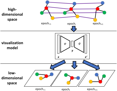
Overview Figure 2 shows an overview of TimeVis solution. In high-dimension space, we consider a superset of representations X = X1 ∪ X2 ∪ ... ∪ Xw . For each sample xti ∈ X, we define its k spatial neighbours and k temporal neighbours. An example of temporal neighbour of xti can be xt+1 i or xt-1 i , i.e., the identical self in the next or previous epoch. By this means, the temporal information is "spatialized". In contrast to spatial neighbours, temporal neighbours can capture the dynamics of a sample in high-dimensional space across epochs. Moreover, the temporal and spatial neighbours are now comparable, which allows us to further capture the relationship of different samples under different epochs.
Based on the defined neighbouring relation, we build a unified spatio-temporal complex for X. Naturally, we only need one visualization model V = ⟨ϕ, ψ⟩ to project between x ∈ X ⊂ Rr and y ∈ Y ⊂ Rl . Note that the same location y in low-dimensional space may have different color (i.e., prediction) in different epoch t according to c = argmaxc∈C ht (ψ(y)). In this work, we use the autoencoder architecture to implement V . Since the temporal relation has been spatialized, the auto-encoder just needs to be trained based loss functions corresponding to the three spatial properties (see Appendix A [Yang et al., 2022a]).
4.1 Spatio-temporal Complex
Spatial Neighbours Given Xt and a distance metric defined on Xt , d(·) : Rr×Rr → R≥0 (e.g., Euclidean distance), we define xti 's k spatial neighbours N S k (xi) = argminJ⊂Xt \{xti },|J|=k ∑xtj ∈J d(xtj , xti ) as its k spatial neighbours.
Temporal Neighbours Given a superset X = X1 ∪X2 ∪ · · · ∪ Xn and a distance metric defined on X, d(·). For a given xti ∈ Xi, we denote its k nearest temporal neighbours as N T k (xti ) = argminJ⊂Xi\{xti },|J |=k ∑xt′ i ∈J d(xt′ i , xti ).
Given an embedding xti ∈ Xi, we use a temporal sliding window with size W to describe its temporal spectrum. In other words, we find its k temporal neighbours N T k (xti ) from the set X′ i = {max(1, xt- W2 i ), . . . , xti , . . . , min(N, xt+ W2 i }). Here, W is an even positive integer, the threshold k and W are the user-defined values.
Spatio-temporal Complex Given the universal superset X = X1 ∪ X2 ∪ · · · ∪ XT , we build the spatio-temporal complex as a graph Gst = ⟨X, Es ∪ Et⟩ where
- the spatial relation set is Es = {(xti , xtj )|xti , xtj ∈ Xt , (xti ∈ N S k (xtj ) or xtj ∈ N S k (xti ))}
- the temporal relation set is Et = {(xtl i , xtm i )|xtl i , xtm i ∈ X, (xtl i ∈ N T k (xtm i ) or xtm i ∈ N T k (xtl i ))}.
For any e = (xtl i , xtm j ) (e ∈ Es ∪ Et), we assign its edge weight as the similarity pitl j tm on the manifold M (See Appendix B for the definition).
Following the training process as in [Yang et al., 2022c] to synthesize boundary points based on the spatial points, train our auto-encoder as the visualization model, we sample the edges in Gst, project the edge ends (i.e., data samples) to
Algorithm 1 Spatial-temporal Complex Construction
Output: reduced spatial-temporal complex, G′st
- 1: for each epoch t ∈ [1, T] do
- 2: Xt′ , E′st = reduce(Xt ,Est )
- 3: end for
- 4: E′t ← ∅
- 5: for each epoch t ∈ [1, T] do
- 6: E′t = E′t ∪ construct_temporal_relation(Xt′ ,W)
- 7: end for
- 8: return G′st = ⟨X1′ ∪ · · · ∪XT ′ ,E′s1 ∪ · · · ∪E′sT ∪E′t⟩
low-dimensional space, and tune the model regarding the loss functions corresponding to the three spatial properties.
4.2 Complex Reduction
It is prohibitively expensive to train a visualization model on the super large spatio-temporal complex when epoch number w and dataset size n are large. The dataset size n is usually much larger than epoch number w (i.e., n ≫ w), meaning the training barrier lies in n.
A spatial-temporal complex Gst can also be written as Gst = ⟨X1 ∪X2 ∪ · · · ∪Xw , (Es1 ∪Es2 ∪ · · · ∪Esw ) ∪Et⟩, where each Est (t ∈ [1,w]) represents the spatial neighbouring relations in epoch et, and Et represents the temporal neighbouring relations among epochs [1,w]. We denote Gt = ⟨Xt ,Est ⟩ as a spatial complex at epoch et. From the perspective of complex construction, reducing the size of each Xt can efficiently leads to the size reduction of Est and Et. It in turn reduces the training cost. In his work, we simplify the complex construction as Algorithm 1. Namely, we reduce each spatial complex regarding the complex structure and reduction size (line 1-3). Then, we build up temporal relations between reduced spatial complex (line 5-7).
Spatial Complex Reduction Given a spatial complex Gs = ⟨X,E⟩, we aim to reduce it to G′s = ⟨X′ ,E′ ⟩ so that (1) Gs and G′s can share as much spatial topological structure as possible and (2) ||X| - |X′ || can be maximized. The former ensures the representativeness of G′s for Gs, and the latter ensures the efficiency of the follow-up complex construction and model training. In this work, we estimate the topological similarity between Gs and G′s by their persistent homology. For self-containment, we provide a brief explanation of persistent homology. Readers can refer to [Chazal et al., 2015; Moor et al., 2020] for more details.
Persistent homology is a concept from topological data analysis (TDA) which describes the topological features on a given point set X where the distance of any pair of points can be evaluated. In topology, a simplice represents a highdimensional topological structure such as point, triangle, tetrahedrons, etc. A simplicial complex K consists of a set of simplices. Let KX be the universal set consisting of all the simplices on X, a filtration is a family of simplicial complexes on KX regarding a distance-based condition C so that:
- Given a distance a, C can be used to slice a subset of simplices Ka ⊂ KX . For example, line segments (1-simplix in hyperspace) of length l ≤ a can be selected to Ka.
Algorithm 2 Greedy Down-sampling Algorithm
Input: a initial sampling size s, a coverage threshold thc, a predefined radius r, a representation set X
Output: a subset X′
- 1: X′ = random_sample(X, s)
- 2: Xc = coverage(X′ ,X, r)
- 3: while |Xc| |X| < thc do
- 4: x′ = k_center_greedy(X \Xc)
- 5: X′ =X′ ∪ {x′ }
- 6: Xc = coverage(X′ ,X, r)
- 7: end while
- 8: return X′
2. For any a ≤ b, Ka ⊆ Kb.
Specifically, a filtration F = {Ka ⊂ KX : a ∈ R≥0}. Given Ka ∈ F, we can derive topological features (e.g., holes) based on its simplices. For example, a topological hole can be constructed by connecting a set of simplices where each simplice x ∈ Ka. Therefore, on X, a topological feature π can appear at distance abirth and disappear at a distance adeath, denoted as life(π) = (abirth, adeath). We define persistent homology on X to track the life span of all the topological features on X. Persistent diagram is a representation of persistent homology where the life span of topological features are represented as dots/lines in a plane.
Given two compact subsets X and X′ from the same metric space X, the bottleneck distance db(DX, DX′ ) of their persistent diagrams DX and DX′ is proved to satisfy the following constraint [Chazal et al., 2016; Chazal et al., 2014]:
The Hausdorff distance dH between X and X′ from the same metric space (X, d) is:
Hence, Hausdorff distance dH(X,X′ ) serves as a upper bound for db(DX,DX′). Therefore, we can transform the spatial complex reduction problem to a search problem to find X′ ⊂ X such that (1) dH(X, X′ ) is minimized and (2) ||X|- |X′ || is maximized. In this work, we design a greedy downsampling algorithm similar to the k center problem [Farahani and Hekmatfar, 2009] to address the issue.
Greedy Down-sampling Algorithm Given radius r, we denote B(x, r) as the ball centered at x with radius r where x ∈ X. We reduce the problem as the search problem for X′ where |X′ | is minimized so that ⋃x′i∈X′ B(x′i , r) can cover X, which is known to be an NP-hard. Hence, we design a greedy down-sampling algorithm to achieve a sub-optimal subset X′ as Algorithm 2.
In Algorithm 2, we first randomly sample s datapoints from X as the initial X′ (line 1). Then, we calculate the coverage set Xc ⊂ X where each x ∈ Xc is covered by ⋃x′∈X′ B(x′ , r). Next, we keep adding into X′ new datapoint from X \ Xc with k-center-greedy algorithm [Gonzalez, 1985] (i.e., selecting the datapoint with largest coverage), until ⋃x′∈X′ B(x′ , r) can cover X regarding user-defined threshold thc. The threshold thc < 1 is set because of the sensitivity of Hausdorff distance to outliers, especially when the input dataset contains noises. Finally, we can achieve a minimized possible X′ most topologically similar to X.
Radius Selection Note that, Algorithm 2 requires a predefined radius, which is adaptive according to the distribution of Xt in the high-dimensional space. Intuitively, the radius should be large when the representations are uniformly distributed in the space (with a larger X′ for X, e.g., in the early training stage). In contrast, the radius can be smaller when the representations are densely clustered in the space (with a smaller X′ for X, e.g., in the late training stage). We use Equation 3 to calculate the radius given the distribution of Xt.
In Equation 3, we first choose a reference epoch e0, then calculate the maximum l2 norm of all representations c0 as a normalization term, and its intrinsic dimension [Facco et al., 2017] d0 as a measurement of representation diversity. Then, we adjust the radius under epoch et with Equation 3. Here, r0, α, and β are user-defined thresholds.
5 Experiment
We evaluate TimeVis with the following research questions. More details are at TimeVis website [Yang et al., 2022b]
- RQ1: Whether TimeVis can faithfully reflect the travelling semantics in high-dimensional space?
- RQ2: How scalable is TimeVis?
- RQ3: While being more temporally reflective and computationally scalable, whether and how TimeVis need to compromise other spatial properties?
Baseline, Datasets, and SubjectModel We choose DVI as our baseline as it is the only time-travelling visualization tool designed to support all spatial and temporal properties. To have a fair comparison, we follow the experiment settings of DVI on selecting datasets and subject models. Specifically, we train ResNet18 on three datasets: CIFAR-10, MNIST, Fashion-MNIST. The high-dimensional representations are extracted from the global average pooling layer (GAP). We visualize all the training epochs of the classifiers on CIFAR10, MNIST and Fashion-MNIST, i.e., 160, 20, and 50.
Visualization Property Measurement We follow the defined spatial and temporal measurements in [Yang et al., 2022c]. Specifically, (1) nnpv(k) for the k spatial neighbour preserving measurement; (2) boundarypv(k) for the k boundary neighbour preserving measurement; (3) recpv for prediction-preserving measurement after a representation is reconstructed from low-dimensional space; and (4) temppv(k) for temporal-preserving measurement of two consecutive epochs.
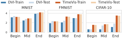
Note that, TimeVis is designed for addressing the accumulated visualization error suffered by DVI, but the temporalpreserving measurement temppv(k) only evaluates temporal continuity between two consecutive epochs. Therefore, we define two more measurements tempg and templ to evaluate how the travelling semantics of each high-dimensional representation are preserved in the low-dimensional space across multiple training epochs. First, we evaluate how many k nearest temporal neighbours of a representation xti can be preserved in the low-dimensional space; Formally, we define templ(i, t, k) as:
where I is the indicating function evaluated to either 0 or 1. Second, we evaluate the correlation of two rankings for any xti . One ranks its temporal neighbours by distance, denoted as r(xti ); the other ranks its the temporal neighbours of its correspondence yt i 'in low-dimensional space by distance, denoted as r(yt i ). Then the tempg is defined as:
We use Euclidean distance as d(·) and Kendall's τ as correlation measurement. Higher tempg(i, t) indicates better preserved semantics, and vice versa.
Runtime Configuration We let TimeVis and DVI share the same auto-encoder architecture, i.e., (r, r2 , r2 , r2 , r2 , 2) and (2, r2 , r2 , r2 , r2 , r) given the feature space dimension as r. We choose W as the epoch length. More configuration details can be referred in the Appendix E [Yang et al., 2022a].
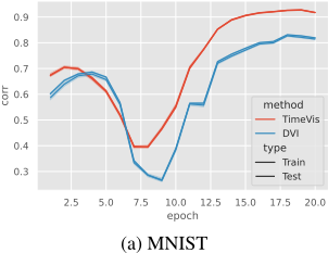
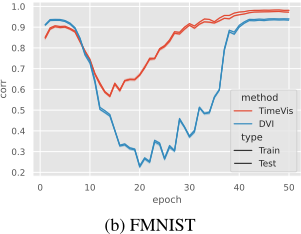
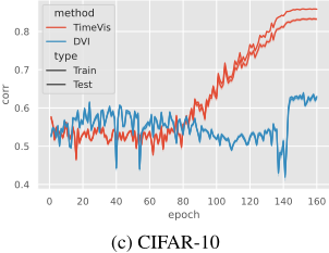
Results (RQ1): Preserving travelling semantics Figure 3 shows that TimeVis improves the travelling semantics in different stages. The Mann-Whitney significance testing on templ(i, t, k) shows that p-value is smaller than 10-5 . Figure 4 further shows how temporal correlation tempg(i, t) of two approaches changes along the training. Overall, TimeVis outperforms DVI, especially in the late training stages.
| Solution | CIFAR-10 | MNIST | FMNIST | |
|---|---|---|---|---|
| TimeVis | CC | 2572.812 | 315.457 | 724.044 |
| training | 1462.170 | 235.887 | 657.353 | |
| overall | 4034.987 | 551.344 | 1381.397 | |
| DVI | overall | 50212.400 | 9563.142 | 22985.150 |
Results (RQ2): Visualization scalability Table 1 shows that, the visualization cost of DVI is ∼15X than TimeVis. Comparing to training the visualization model for each recorded classifier, TimeVis only needs to train the visualization model for once.
| Solution | CIFAR-10 | MNIST | FMNIST | |||
|---|---|---|---|---|---|---|
| train | test | train | test | train | test | |
| TimeVis | -0.268 | -0.267 | -0.542 | -0.543 | -0.162 | -0.164 |
| DVI | -0.240 | -0.238 | -0.470 | -0.470 | -0.318 | -0.316 |
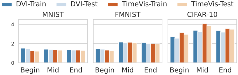
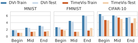
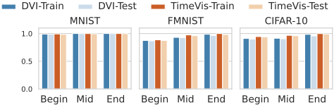
Results (RQ3): Potential compromise Figure 5, Figure 6, Figure 7, and Table 2 compare the performance between TimeVis and DVI. We can see that they are comparable in the measurements of neighbour preserving and prediction preserving rate. However, DVI outperforms TimeVis regarding boundary distance preserving property. We will enhance TimeVis by improving the integration of the boundary points into the spatio-temporal complex in the future work.
6 RelatedWork
Visual Explanation of Deep Models Many research works have been proposed to provide visual explanations to deep models, including activation maps [Alsallakh et al., 2021; Zeiler and Fergus, 2014] and attribution methods [Adebayo et al., 2018]. Particularly, IntGrad [Sundararajan et al., 2017] and ACE [Chattopadhyay et al., 2019] are the pioneering work in the area. TimeVis focuses on visualizing the training dynamics, which is complementary to those tools to understand the behaviors of deep models.
Dimension Reduction Dimension reduction methods are widely used for visualizing the high-dimensional feature vectors. Existing techniques can be divided into parametric ones (e.g., Topological Autoencoder [Moor et al., 2020], VAE-SNE [Graving and Couzin, 2020], parametric UMAP [Sainburg et al., 2021]) and non-parametric ones such as UMAP [McInnes et al., 2018].
They are the pioneering work to derive time-travelling visualization. Comparing to those techniques on visualizing a "snapshot", time-travelling visualization generates "animation" to understand the model training process.
Time-travelling visualization DVI [Yang et al., 2022c] first proposes three spatial and one temporal properties for any time-traveling visualization methods and trains auto-encoders to fulfill all properties. However, DVI still suffers from large visualization cost and accumulative visualization errors. TimeVis is proposed to addresses the above two problems.
7 Conclusion
We propose TimeVis, a temporality-spatialization based timetravelling visualization approach. TimeVis constructs a unified spatio-temporal complex which captures spatial and temporal neighbours of any high-dimensional samples. TimeVis improves the state-of-the-art solution DVI both in training efficiency and visualization faithfulness. In the future, feedback-based solutions [Lin et al., 2017], trace alignment based solutions [Wang et al., 2019], and input manipulation based solution [Xiao et al., 2021] will be designed to improve tool usability and extensibility;
Acknowledgements
This research is supported in part by the Minister of Education, Singapore (T2EP20120-0019, T1-251RES1901, MOET32020-0004), and A*STAR, CISCO Systems (USA) Pte. Ltd and National University of Singapore under its Cisco-NUS Accelerated Digital Economy Corporate Laboratory (Award I21001E0002)
@inproceedings{ijcai2022p558,
  title     = {Temporality Spatialization: A Scalable and Faithful Time-Travelling Visualization for Deep Classifier Training},
  author    = {Yang, Xianglin and Lin, Yun and Liu, Ruofan and Dong, Jin Song},
  booktitle = {Proceedings of the Thirty-First International Joint Conference on
               Artificial Intelligence, {IJCAI-22}},
  publisher = {International Joint Conferences on Artificial Intelligence Organization},
  editor    = {Luc De Raedt},
  pages     = {4022--4028},
  year      = {2022},
  month     = {7},
  note      = {Main Track},
  doi       = {10.24963/ijcai.2022/558},
  url       = {https://doi.org/10.24963/ijcai.2022/558},
}
TY - CPAPER TI - Temporality Spatialization: A Scalable and Faithful Time-Travelling Visualization for Deep Classifier Training AU - Yang, Xianglin AU - Lin, Yun AU - Liu, Ruofan AU - Dong, Jin Song T2 - Proceedings of the Thirty-First International Joint Conference on Artificial Intelligence, IJCAI-22 PB - International Joint Conferences on Artificial Intelligence Organization PY - 2022 SP - 4022 EP - 4028 DO - 10.24963/ijcai.2022/558 UR - https://doi.org/10.24963/ijcai.2022/558 ER -Copied
Machine-readable versions of this paper, for tools and AI agents:





