Budgeted Sequence Submodular Maximization

1 Introduction

Submodular optimization is a fundamental optimization problem [Fujishige, 2005] which can be used in many applications. Most existing studies focus on the problem of selecting a subset of items from a whole set in order to maximize a given submodular function over the set, such as influence maximization [Kempe et al., 2003] and information gathering [Leskovec et al., 2007].

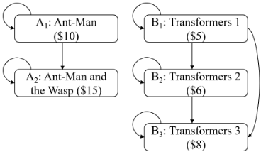
In many applications, the order of selecting items affects the utility of item sets, and thus it is desired to select a sequence of items instead of a subset. In Fig. 1, we use an example of movie recommendations to explain why sequence selection is meaningful and useful. Assume that a utility function over a sequence of movies measures how users are satisfied with these recommendation results. We can use the directed edges between two movies to represent that there is an additional utility in watching them by following the order, and the self-cycles to represent the utilities of watching individual movies. It can be observed that the order of watching movies affects users' experience. For example, watching B2 : Transformers 2 after B1 : Transformers 1 has a higher utility than watching the two movies in reverse order.

∗Liang Feng is the corresponding author.

This interesting observation commonly occurs in recommender systems [McAuley et al., 2015], paper reading plan [Shahaf et al., 2012], course learning [Parameswaran et al., 2011], etc. Thus, the problem of selecting a sequence of items that maximizes a given submodular function over the sequence has recently received increasing attention [Tschiatschek et al., 2017; Qian et al., 2018; Mitrovic et al., 2019; Sallam et al., 2020].

In many submodular optimization problems, the items have non-uniform costs [Khuller et al., 1999; Bian et al., 2020; Amanatidis et al., 2020]. In sequence selection, non-uniform item costs are common as well. For instance, in the movie recommendation example, movies could have different costs (e.g., their DVD prices); in the course sequence design, costs (i.e., the time cost) of courses are also non-uniform. In addition, users may have a budget limit on the sequence recommended to them. However, all existing studies on sequence selection only consider uniform costs of items (i.e. cardinality constraints), although non-uniform costs of items are more general in many real-world applications.

In this paper, we study the problem of Budgeted Sequence Submodular Maximization (BSSM) by considering non-uniform costs of items, and prove the NP-hardness of the BSSM problem. The BSSM problem adapts the sequence submodular function proposed by Tschiatschek et al. [Tschiatschek et al., 2017], as the function is more expressive and it can capture the effect of the order of items in the sequence on the utility of item sets. Note that the sequence submodular function of BSSM is submodular on the sequences, but not on items. Hence, a simple greedy algorithm that selects one item in each iteration greedily cannot return results with a guaranteed error bound [Tschiatschek et al., 2017].

Due to non-uniform costs of items, the state-of-the-art algorithm OMEGA [Tschiatschek et al., 2017] for sequence selection with uniform costs always obtains sequences with poor quality (as shown in the experimental study). To solve this problem, we propose a greedy algorithm GBM which picks an edge with the largest marginal cost-effective value, and we prove its error bound by exploiting the properties of the sequence submodular function.

Similar to traditional greedy algorithms, GBM often gets trapped at local optima in the search space. To address this issue and improve the algorithm effectiveness, we develop an anytime algorithm POBM based on Pareto optimization. POBM first reformulates the original constrained optimization problem as a bi-objective optimization problem that maximizes the objective function f and minimizes the cost function C simultaneously, then utilizes a randomized iterative method to solve it, and finally selects the best feasible solution from the maintained set of solutions. Our theoretical analysis shows that POBM not only obtains approximation solutions in expected polynomial running time, but also has chances to find the optimal solution. In addition, POBM has a faster expected rate of convergence compared to the state-of-the-art algorithm POSEQSEL [Qian et al., 2018] for Sequence Submodular Maximization with Cardinality Constraints (SSMCC).

In summary, our main contributions are fourfold. Firstly, we propose the BSSM problem and show its NP-hardness. Secondly, we develop a greedy algorithm GBM, and an anytime algorithm POBM with some optimizations to solve this problem. Thirdly, we theoretically analyze the approximation ratio of GBM, and prove that POBM can achieve the same approximation guarantee as GBM in a reasonable time and can escape from the local optimum. Finally, we conduct experiments on both synthetic and real-world datasets to demonstrate the effectiveness and efficiency of our proposed algorithms. Due to space limitations, the proofs of all theorems and some additional experimental results are presented in the extended version of this paper 1 .

2 RelatedWorks

Submodular Optimization. Submodular optimization has been studied substantially due to its wide range of applications including viral marketing [Kempe et al., 2003], information gathering [Leskovec et al., 2007], deep neural network training [Joseph et al., 2019], region search [Chen et al., 2020] etc. A classical problem of submodular optimization is to maximize a non-negative monotone submodular function under cardinality constraints. To solve this problem, Nemhaser et al. [Nemhauser et al., 1978] proposed a simple greedy algorithm with a constant factor approximation ratio of 1 - e-1 and Das et al. [Das and Kempe, 2011] further improved the approximation ratio by introducing a submodular ratio. Meanwhile, different types of generalizing submodular optimization have been the focus of many studies recently. For instance, there exist non-monotone submodular maximization [Amanatidis et al., 2020], streaming submodular maximization [Halabi et al., 2020], and continuous submodular maximization [Raut et al., 2021], and so on. These studies aim to select a subset of items rather than a sequence.

1 https://xincao-unsw.github.io/attaches/pubs/BSSM-Full.pdf

Sequence SubmodularMaximization. Many studies have considered sequence submodular maximization, since the sequence plays an important role in submodular optimization applications. Aliaei et al. [Alaei et al., 2010] first considered sequence selection in submodular maximization by introducing non-decreasing sequence submodular functions. Zhang et al. [Zhang et al., 2015] presented a string submodular function by relaxing the sequence-submodular function. These two submodular functions fail to consider the effect of the order of items in the sequence on the functions. To fill this gap, Tschiatschek et al. [Tschiatschek et al., 2017] proposed a new class of sequence submodular functions on a directed graph. As this function is expressive, it has been used to study the submodularity on a hypergraph [Mitrovic et al., 2018] and adaptive sequence submodularity [Mitrovic et al., 2019]. To solve all the above problems of sequence submodular maximization, Qian et al. [Qian et al., 2018] proposed an algorithm POSEQSEL based on Pareto optimization. Meanwhile, Sara et al. [Bernardini et al., 2020] offered a unified view of sequence submodularity, and Gamal et al. [Sallam et al., 2020] first studied the problem of robust sequence submodular maximization. However, these works only consider uniform costs (i.e. cardinality constraints).

Submodular Optimization with Non-uniform Costs (Knapsack Constraint). Although uniform costs have been used extensively in existing submodular optimization studies, non-uniform costs are more general in real-world applications. Khuller et al. [Khuller et al., 1999] proposed a budgeted maximum coverage problem which first considered non-uniform costs in submodular optimization, and they developed a greedy algorithm with an error bound. Sviridenko [Sviridenko, 2004], Krause and Guestrin [Krause and Guestrin, 2005] presented efficient approximation algorithms for the budgeted maximization of nondecreasing submodular set functions. Georgios et al. [Amanatidis et al., 2020] designed a fast randomized greedy algorithm that achieves a 5.83 approximation for non-monotone submodular maximization subject to a knapsack constraint. In recent years, Qian et al. [Qian et al., 2017] considered a general cost constraint on a subset selection which is a type of submodular maximization, and proposed POMC algorithm based on Pareto optimization for the problem. To solve the problem more effectively, Bian et al. [Bian et al., 2020] developed a new anytime algorithm EAMC with a better approximation ratio. None of the existing work considers non-uniform costs of items for sequence submodular maximization.

3 ProblemFormulation

In this section, we formally define the problem of Budgeted Sequence Submodular Maximization (BSSM) and show its NP-hardness. Here, we adapt the sequence submodular setting [Tschiatschek et al., 2017], as it considers the effect of the order of items in the sequence on the utility of item sets [Tschiatschek et al., 2017; Mitrovic et al., 2018]. We first present the sequence submodular setting as below.

Definition 1. Item Sequences. Given a set of n items V = (v1, v2, · · · , vn), a sequence from V is represented as s = {(s1, s2, · · · , sk)|si ∈ V, k ∈ Z+}, and s ∈ S, where S is the set of all possible sequences of items from V , and k = 0 represents the empty sequence ∅. For two sequences s and t, their concatenation is denoted as s ⊕ t.

The utility function of sequences can be defined through a directed graph G = (V, E) where vertices correspond to the items V , and a set of edges E represents the utility in picking items in a certain order. An example of G is shown in Fig. 1. Specifically, the edge eij = (vi, vj) represents the utility in selecting vj after vi, and the self-cycle eii(vi, vi) represents the utility of selecting vi individually. We define the utility function as below.

where E(s) = {(si, sj)|(si, sj) ∈ E, i ≤ j} is the set of edges induced by the sequence s, and h : 2E → R+ is a nonnegative monotone submodular set function over the edges. It means that for an edge e ∈ E, h(E1 ⋃{e}) - h(E1) ≥ h(E2 ⋃{e}) - h(E2) if E1 ⊆ E2 ⊆ E and e /∈ E1.

However, the utility function f is neither a set function nor submodular on items. We use an example to explain this. As shown in the example of Fig. 1, and assume that h(E(s)) counts the number of edges in E(s), and thus the utilities of the sequences(A1), (A2), (A1,A2) and (A2,A1) are computed as:

Note that the order of selecting items affects the utilities of item sets, i.e., f((A1,A2)) ̸= f((A2,A1)), and the function f is not submodular over item sets, because f((A1))-f(∅) ≱ f((A1,A2)) - f((A2)) although ∅ ⊂ A2 (i.e., it does not satisfy the diminishing returns property). On the other hand, the function f is more expressive than submodular functions over items. This is because, when the graph G only has selfcycles and no other edges, f can express any submodular set function.

Besides the utilities of sequences, we consider the costs of sequences, and we define the cost score of a sequence as the sum of the costs on all items in the sequence, which is computed as: C(s) = ∑vi∈s cvi , where cvi is the cost of vi. Formally, we define the BSSM problem as follows:

Definition 2. Budgeted Sequence SubmodularMaximization (BSSM). Given a set of n items V = (v1, v2, · · · , vn)

with item costs (cv1 , cv2 , · · · , cvn ), a utility function f over the sequences of items, and a budget constraint ∆, the target is to find a sequence s such that

For example, consider the instance of movie recommendation in Fig. 1 again. Given ∆ = 20, the optimal sequence of the BSSM problem is (B1,B2,B3), as it allows the user to fully enjoy three movies under the budget constraint.

Theorem 1. The BSSM problem is NP-hard.

4 The GBMAlgorithm

In this section, we propose a novel greedy algorithm called GBM for solving the BSSM problem and prove its error bound. Instead of picking the edge with the maximum marginal utility (which is conducted by OMEGA [Tschiatschek et al., 2017]), GBM chooses the edge with the maximum marginal cost-effective value in each step until no more edges can be inserted into the solution. This can guarantee the approximation ratio of GBM.

As shown in Alg. 1, GBM starts by initializing a candidate edges set Eca and an edge set Ese for storing the selected edges (line 1). After that, the algorithm iteratively and greedily extends Ese until no more edges can be added (lines 2-6). In each iteration, the algorithm first updates Eca by pruning the edges whose all vertexes (i.e., items) belongs to V (Ese ) or would make the cost of the selected edge set exceed the budget constraint (lines 3-4). Next, it selects the edge e∗ with the maximum marginal cost-effective value ∆f/∆C = f(RE(Ese∪{el}))-f(RE(Ese ))

C(Ese∪{el})-C(Ese ) to insert into Ese (lines 5-6), where C(Ese ) = ∑vi∈V (Ese ) cvi , V (Ese ) denotes the set of items in Ese , and RE(Ese ) is a function for obtaining the optimal order with the maximal value of the utility function over all possible orders of items contained in Ese (i.e., RE(Ese ) = REORDER(Ese ), and the algorithm of implementing function REORDER is shown in the previous work [Tschiatschek et al., 2017]). After finishing the extension of Ese , the algorithm obtains the best sequence s1 in Ese

Algorithm 1: GBM Algorithm

Input: G = (V, E), a utility function f , item costs (cv1 , cv2 , · · · , cvn ), ∆ Output: A sequence s 1 Eca ←E, Ese ← ∅; 2 while Eca ! = ∅ do 3 Eca ←Eca \ {el = (vi, vj)|vi, vj ∈ V (Ese )}; 4 Eca ←Eca \ {el ∈ Eca |C(Ese ∪ {el}) >∆} ; 5 e∗ ← argmaxel∈Eca f(RE(Ese ∪{el}))-f(RE(Ese )) C(Ese∪{el})-C(Ese) ; 6 Ese ←Ese ∪ {e∗ }; 7 s1 ←RE(Ese ); 8 e′ ← argmaxel∈E,C(el)≤∆f(RE(el)); 9 s2 ←RE({e′ }); 10 s ← argmaxsi∈{s1,s2}f(si ); 11 return the sequence s;

using RE(Ese ) (line 7). It also gets another sequence s2 that only has one edge with the maximal utility and satisfies the budget constraint (lines 8-9). Finally, it returns the sequence with the largest utility as the solution s.

We obtain the approximation ratio of GBM in Theorem 2. For the sake of clarity, we let cmin = minvi∈V cvi and introduce a parameter β = 4⌊ ∆ cmin ⌋.

Next, we analyze the complexity of GBM. It requires ⌊ ∆ cmin ⌋ iterations in the worst case, and in each iteration, it takes O(n2 ) time to update Eca , and costs O(n2 ⌊ ∆ cmin ⌋log⌊ ∆ cmin ⌋) time to select the edge e∗ for inserting into Ese , since the number of items in Ese is less than ⌊ ∆ cmin ⌋ and the complexity of computing f(RE(Ese )) is O(⌊ ∆ cmin ⌋log⌊ ∆ cmin ⌋). And then, GBM costs O(⌊ ∆ cmin ⌋log⌊ ∆ cmin ⌋)) time and O(n2 ) time to obtain s1 and s2 , respectively. Thus, the time complexity of GBM is O(n2 (⌊ ∆ cmin ⌋)2 log⌊ ∆ cmin ⌋).

5 The POBMAlgorithm

Although GBM can achieve an approximate solution in a reasonable time, it usually gets trapped in a local optimum due to the greedy rule. To alleviate this issue, we design an anytime algorithm POBM based on Pareto Optimization [Qian et al., 2015]. For POBM, most of its steps are similar to those of POMC [Qian et al., 2017] which is for the problem of subset selection with a general cost constraint. But POBM uses a different objective function and adopts the function RE (which is mentioned in the above section) to obtain the best sequence from an item set. Note that the input of function RE can be an item set or an edge set.

Let a Boolean vector p ∈ {0, 1}n represent an item set, and C(p) = ∑vi∈p cvi . POBM reformulates BSSM as a bi-objective maximization problem.

and f2(p) = -C(p). It means that POBM maximizes the utility function f and minimizes the cost function C simultaneously. By setting f1 to -∞, we exclude overly infeasible solutions. In the bi-objective setting, we consider both the two objective scores to compare two item sets p and p′ . p weakly dominates p′ (i.e., p is better than p′ , denoted as p ⪰ p′ ) if f1(p) ≥ f1(p′ ) and f2(p) ≥ f2(p′ ); p dominates p′ (i.e., p is strictly better than p′ , denoted as p ≻ p′ ) if p ⪰ p′ and either f1(p) > f1(p′ ) or f2(p) > f2(p′ ). But if neither p is better than p′ nor p′ is better than p, they are incomparable.

The procedure of POBM is presented in Alg. 2. It begins with initializing a solution set P by adding the empty item set {0}n into it (line 1). In the following steps, it iteratively tries to improve the quality of the item sets in P (lines 2-9).

Algorithm 2: POBM Algorithm

Input: G = (V, E), a utility function f , item costs (cv1 , cv2 , · · · , cvn ), ∆, the number T of iterations Output: A sequence s 1 p← {0}n , P ← {p}, t ← 0; 2 while t < T do 3 Obtain p fromP uniformly at random; 4 Generate p′ by flipping each bit of p with prob. 1n ; 5 if ∄z ∈ P such that z ≻ p′ then 6 P ← (P \ {z ∈ P |p′ ⪰ z}) ∪ {p′ }; 7 t = t + 1; 8 pbe ← argmaxp∈P,C(p)≤∆f(RE(p)); 9 s ←RE(pbe ); 10 return the sequence s;

In each iteration, a new item set p′ is generated by randomly flipping bits of an archived item set p selected from the current P randomly (lines 3-4); if p′ is not dominated by any archived item set in P, it will be inserted into P, and meanwhile, the archived item sets which are weakly dominated by p′ will be pruned from P (lines 5-6). Obviously, P always contains incomparable item sets. After T iterations, the algorithm obtains the best feasible item set pbe with the maximum utility score from P, and then gets the best sequence s from pbe to return as a solution (lines 8-10).

The number T of iterations affects the solution quality of POBM, we analyze their relation in a theoretical way, and achieve the approximation ratio of POBM in Theorem 3, where E(T ) denotes the expected number of iterations, Pmax denotes the largest size of P during the running process of POBM, and s∗ denotes an optimal sequence. Generally, we set cvi ∈ Z+ for each vi ∈ V , thus Pmax ≤ 2∆.

Theorem 3. When G is a DAG (not counting self-cycles), POBM with E(T) ≤ ⌊ ∆

Theorem 3 shows that POBM can obtain the same approximation ratio as GBM. Next, we explain that POBM has chances to find a global optimum in the following theorem.

Algorithm POSEQSEL [Qian et al., 2018] which is proposed for SSMCC is also an anytime algorithm based on Pareto Optimization. We observe that POSEQSEL can be adopted to solve BSSM after replacing its two objective functions with those of POBM. We analyze the approximation ratio of POSEQSEL in BSSM and get the following Theorem.

Theorem 5 illustrates that, compared to POSEQSEL, POBM has a better expected rate of convergence for achieving the approximate solution. We will further verify it in the experimental study.

Since POBM is an anytime randomized iterative algorithm, it would consume a lot of time when the number of iterations is large. To improve the efficiency of POBM Algorithm, we present two optimizations: speeding up computing E(RE(p)) and the quick dominance check.

We first speed up computing E(RE(p)). As p′ is generated by flipping each bit of p with probability 1n , there is one different bit between p′ and p in average. Thus, we can reuse E(RE(p)) to compute E(RE(p′ )) quickly in two steps.

In step 1, we obtain the items in p and not in p′ (i.e., pde = {vi ∈ p \ p′ }), and then delete all edges which has an item in pde from E(RE(p)) (i.e., Es1 = E(RE(p)) \ Ede and Ede = {(vi, vj)|vi ∈ pde ||vj ∈ pde }).

In step 2, we first achieve the items in p′ and not in p (i.e., pad = {vi ∈ p′ \ p}). After that, we get the edges among items in pad , and between items in pad and items in p \ pde (i.e., Ead = {(vi, vj)|vi, vj ∈ pad ||vi ∈ pad , vj ∈ p\pde }). Finally, we can obtain E(RE(p′ )) by combining Es1 and Ead (i.e., E(RE(p′ )) = Es1 ∪ Ead )

Next, we describe the optimization for the quick dominance check. For each new solution, POBM needs to do a dominance check, and then delete all weakly dominated solutions if the new solution is not dominated by any solution in the archive P. To accelerate this process, we first sort the solutions in P in ascending order of their cost scores. After that, we can only use the solution p that has the closest cost score to the new solution p′ and C(p) ≤ C(p′ ) to check whether p′ is dominated by any solution in P. If not, we insert p′ into P, and then check p and the solutions after p in P one by one and delete the weakly dominated solutions, until the solution's utility score is larger than that of p′ or all solutions are scanned.

Remarks. If the graph G is not a DAG, GBM and POBM can still be used for BSSM, as function RE can get approximate orders by computing a feedback vertex set of G [Karp, 1972]. Although the theoretical guarantees cannot hold in this case, GBM and POBM can also achieve high-quality solutions, which is demonstrated in the experimental study.

6 Experimental Study

In this section, we study the experimental performance of our algorithms using both synthetic and real-world datasets. We denote POBM with the optimizations of speeding up computing E(RE(p)) and the quick dominance check as POBMOpt. We use two state-of-the-art algorithm for SSMCC (i.e., OMEGA [Tschiatschek et al., 2017] and POSEQSEL [Qian et al., 2018]) as baseline methods. We implement all the algorithms in C++ on Windows 10, and run on a desktop with an Intel(R) i7-10700 2.9 GHz CPU and 32 GB memory.

6.1 Synthetic Datasets

Datasets and Parameter Settings

We generate the synthetic datasets following the previous work [Tschiatschek et al., 2017; Qian et al., 2018] for the problem of sequence selection. We first construct the graph G = (V,E) as follows: for each item vi ∈ V , select a subset of size min{d, n - i} uniformly at random from {vi+1, · · · , vn}, where d is the maximum out-going degree of the graph, and then build an edge from vi to each item in the selected subset and to itself (self-cycles). To assign a utility wi,j to each edge (vi, vj), we consider two sets of functions h : 2E → R+, one is modular with h(E(s)) = ∑(vi,vj)∈E(s) wi,j, and the other one is submodular with h(E(s)) = ∑vj∈V (E(s)) [1 - ∏(vi,vj)∈E(s) (1 -wi,j)]. For the modular h, we get each utility wi,j by sampling from [0, 1] randomly. For the submodular h, we get each utility wi,j with i < j by sampling from [0, 1] randomly, and each utility wi,i by sampling from [0, 0.1] randomly. We obtain the cost cvi for each item vi ∈ V by sampling the values from {1, 2, 3, 4, 5} randomly. To compute the approximation ratios of algorithms, we use an exhaustive enumeration to find the optimal solutions and set n = 50, B = 10 by default. For each experiment, we generate 50 problem instances randomly and report the average results.

(b) Submodular h

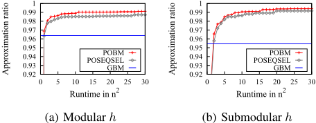
Figure 3: The effect of T on the solution quality for POBM and POSEQSEL over modular and submodular utility functions.

Performance of Our Methods

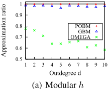
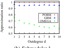
We first compare GBM and POBM with OMEGA in terms of the solution quality by varying maximum outdegree d from 1 to 10, as the proposed optimizations do not affect the solution quality. We set the number T of iterations of POBM as 2∆⌊ ∆ 2cmin ⌋en2 , that is suggested by Theorem 3. The approximation ratios of the three algorithms are shown in Fig. 2. It illustrates that GBM and POBM can achieve high-quality solutions, while the solution quality of OMEGA is poor, as OMEGA is designed for the uniform cost setting. POBM outperforms other algorithms and almost finds the optimum.

Next, we investigate the effect of T on the solution quality for POBM and POSEQSEL in both modular and submodular utility functions with d = 5. Fig. 3 shows the curve of the approximation ratio over time for POBM and POSEQSEL by using GBM as the baseline. It demonstrates that POBM and POSEQSEL can quickly find a better solution whose approximation ratio is more than 95%, and POBM converges faster than POSEQSEL, which is consistent with the theoretical analysis. Note that the results of GBM keep unchanged, as they are not affected by T. According to this result, we set T = 10n2 for POBM by default. Note that the result of examining the acceleration of our optimizations on POBM is reported in the extended version of this paper.

6.2 Two Real-world Datasets

Datasets and Parameter Settings

We use two real-world datasets, one is the Movielens 1M (MOV) dataset [Harper and Konstan, 2015] and the other one is the XuetangX (XTX) dataset [Feng et al., 2019]. MOV contains 1, 000, 209 time-stamped ratings made by 6, 040 users for 3, 706 different movies in MovieLens platform, and XTX has the tracking log files that records the 772, 887 users' learning behavior over 1, 629 courses in XuetangX platform from August 2015 to August 2017. They will be used to do a movie recommendation and a course sequence design task, respectively. In order for our data to be representative of the general population, referring to the work [Mitrovic et al., 2018], we preprocess those datasets and then obtain 412, 222 ratings made by 2, 549 users for 882 different movies in MOV, and the tracking log files made by 238, 834 users' over 956 courses in XTX.

Following the work [Tschiatschek et al., 2017], we use the utility function h(E(s)) = ∑vj∈V (E(s)) [1 - ∏(vi,vj)∈E(s) (1 - pj|i)], where pj|i associated on the edge (vi, vj) is the conditional probability that a user rates movie (or enrolls course) vj given that she has rated movie (or enrolled course) vi before, and pi|i associated on self-cycles is the item frequency pi. We next construct the graph G = (V,E) to compute pj|i referring to the work [Tschiatschek et al., 2017]. We also obtain the cost cvi for each movie by crawling the purchase price from Amazon's website, and extract the costs of courses from the XTX dataset directly.

Performance of Our Methods

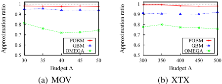
We first compare GBM and POBM with OMEGA in terms of the solution quality on both MOV and XTX datasets by varying the budget constraint. To compute the approximation ratios of algorithms, we use an exhaustive enumeration to find the optimal solutions and sample 50 movies (or courses) randomly for each instance (i.e., n = 50). And we generate 50 problem instances randomly and report the average results. As shown in Fig. 4, although the worst-case error bound of GBM is poor, GBM can obtain high-quality solutions, and POBM nearly achieves the optimal solutions.

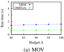
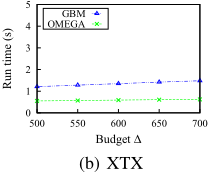
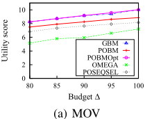
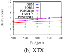
To further compare the performance of these algorithms, we run them on the entire MOV and XTX datasets with larger ∆ to solve the problem. The run time of GBM and OMEGA on both datasets is shown in Fig. 5. As POBM, POBMOpt and POSEQSEL require a large number of iterations when the number of items n is large, we set a time limit TimLim = 30s for them to compare their solution quality with that of GBM and OMEGA. As shown in Fig. 6, in terms of the solution quality, POBMOpt > POBM > POSEQSEL, it demonstrates that, our optimization can speed up POBM well, and POBM has a faster rate of convergence than POSEQSEL. Note that GBM can achieve high-quality solutions within 2s when ∆ is large, and the solution quality of POBMOpt is always the best on both datasets.

7 Conclusion

We propose the BSSM problem which aims to find the optimal sequence such that it maximizes the utility of the sequence computed by a sequence submodular function under a given budget constraint. The problem is proved to be NPhard. To solve the BSSM problem, we propose a greedy algorithm GBM and an anytime algorithm POBM based on Pareto optimization. We also analyze the approximation ratios of GBM and POBM, and present some optimizations to speed up POBM. The results of empirical studies on both synthetic and real-world datasets verify the theoretical analysis and show that our proposed algorithm can perform well in practice. In future work, would like to focus on the theoretical development of a parallel POBM.

Acknowledgments

This work was supported in part by NSFC Grants (No. 61876025, 61836005, 62176225, and 61906032), the Fundamental Research Funds for the Central Universities under Grant DUT21TD107, and ARC DE190100663.