Generalisation of Alpha-Beta Search for AND-OR Graphs With Partially Ordered Values

1 Introduction

Search in graphs containing AND- and OR-nodes is used as a basis of many algorithmic solutions to Artificial Intelligence problems. In such graphs, OR-nodes typically model choice nodes where an agent can choose a successor, while ANDnodes model an opponent. For instance, in robust planning with nondeterministic actions, an AND-node models the outcome of an action: a strategy must be valid whatever the outcome [Kissmann and Edelkamp, 2009]. Similarly, when solving a zero-sum two-player (sequential) game for a player, OR-nodes are those at which it is her turn to play, while AND-nodes correspond to her opponent [Van Den Herik et al., 2002]: the value of an OR-node is 1 if and only if at least one move leads to a node with value 1; dually, at ANDnodes, the values of the children are conjoined. More generally, in games that can have more than two outcomes, such as chess or checkers [Schaeffer et al., 2007], AND-nodes (respectively OR-nodes) correspond to a minimum (respectively maximum) operator on the values of their children.

A fundamental question is that of evaluating rooted ANDOR directed acyclic graphs (DAGs), which means computing the value of their root given a value for each of their leaves. For instance, in games with complete information, selecting the best move for the current turn amounts to evaluate each of the children of the root. This problem has been thoroughly studied in the literature [Marsland, 1986] under the setting of totally ordered values (Boolean or real) and the standard AND/OR or min/max operators. Following [Ginsberg and Jaffray, 2002], we investigate here a more general setting, where the values are taken from a distributive lattice (V, ∧, ∨) (i.e. a partially ordered set with least upper bound and greatest lower bound for any two elements), and operators for AND- and OR nodes are taken to be the meet ∧ and join ∨, respectively. This setting arises naturally in many applications, in particular in games with incomplete information. Example of such games are Skat [Kupferschmid and Helmert, 2006; Rebstock et al., 2019; Edelkamp, 2020], Bridge [Levy, 1989; Ginsberg, 2001; Cazenave and Ventos, 2020], Hearts and Spades [Sturtevant and White, 2006].

∗A long version with full proofs is available at the URL https: //hal.archives-ouvertes.fr/hal-03656224.

A well-known technique for evaluating AND-OR graphs is alpha-beta pruning, which maintains a lower bound α (respectively upper bound β) on the value of each OR-nodes (respectively AND-nodes), and uses them to prune some of their successors. This technique is currently used in strong chess programs [Haworth and Hernandez, 2021] combined with sophisticated evaluation functions such as NNUE neural networks that were first used in Shogi [Nasu, 2018]. However, the generalisation of alpha-beta pruning to AND-OR DAGs with partially ordered values is nontrivial since two values from a lattice are not always comparable. We build on the seminal work by [Ginsberg and Jaffray, 2002] and generalise it by proving the correctness of lattice-valued alpha-beta pruning with the consideration for heuristic functions.

Orthogonally, we investigate caching techniques for alphabeta pruning in lattice-valued DAGs. The question is again nontrivial because nodes are in general revisited with different α and β than during previous visits. For this, we propose a new algorithm called 'alpha-beta duo'. We state its correctness and experimentally evaluate its efficiency.

The paper is organised as follows. Preliminaries are given in Sections 2 and 3. We extend the work by [Ginsberg and Jaffray, 2002] in Section 4, and present alpha-beta duo in Section 5. We then report experimental results and conclude.

2 Preliminaries

The following definitions on posets and lattices are based on [Davey and Priestley, 2002].

Definition 1. Let V be a set and ⪯ be a binary relation on V . Then (V, ⪯) is called a partially ordered set (poset) if ⪯ is a partial order (i.e. reflexive, transitive, and antisymmetric).

For a poset (V, ⪯) and S ⊆ V , an element x ∈ V is called an upper bound (UB) of S if s ⪯ x holds for all s ∈ S, and x is called a least upper bound (LUB) if in addition x ⪯ y holds for any UB y of S. If S has an LUB, then it is unique. The greatest lower bound (GLB) of S is defined dually. For x, y ∈ V , we write x ∨ y ('x join y') and x ∧ y ('x meet y') respectively for the LUB and GLB of {x, y}, when they exist.

Definition 2. A poset (V,⪯) is called a distributive lattice if

• for all x, y ∈ V , x ∨ y and x ∧ y exist,
• for all x, y, z ∈ V , x ∨ (y ∧ z) = (x ∨ y) ∧ (x ∨ z),
• for all x, y, z ∈ V , x ∧ (y ∨ z) = (x ∧ y) ∨ (x ∧ z).

It is moreover said to be bounded if there are elements ⊥, ⊤ ∈ V satisfying ⊥ ⪯ x and x ⪯ ⊤ for any x ∈ V .

In the remainder of this paper, we denote by (V,⪯, ∧, ∨) an arbitrary bounded distributive lattice.

Example 1. Let S be a set and let 2S denote its powerset. Then (2S ,⊆, ∩, ∪) is a bounded distributive lattice with set inclusion ⊆ as partial order, set intersection ∩ and set union ∪ respectively as meet and join, ∅ as ⊥, and S as ⊤.

We denote any directed acyclic graph (DAG) by G = (N,C), where N is the set of nodes, and C : N → 2N is a function that yields the set of children of each node. A root r is a node without predecessor (i.e. for any n ∈ N, r /∈ C(n)), and a leaf is a node without child. We denote the set of leaves of a DAG G by LG. We only consider rooted DAGs, which contain a (necessarily unique) root r such that there exists a directed path to every vertex from r.

An AND-OR DAG is a rooted DAG (N,C, r) equipped with a labelling function ℓ : N → {A, O}. Nodes labelled by A and O are respectively called AND-nodes and OR-nodes. Note that we do not impose nodes to be alternating.

3 Problem Setting

We are interested in the problem of evaluating the root value of an AND-OR DAG, given values for all its leaves. Formally, given an AND-OR DAG G = (N, C, r, ℓ), a bounded distributive lattice (V,⪯, ∧, ∨), and an evaluation function e : LG → V assigning a value in V to each leaf of G, the goal is to compute v(r), where the value v(n) of n ∈ N is defined recursively by:

• for a leaf node n, v(n) := e(n);
• for an internal AND-node n, v(n) := ∧c∈C(n) v(c);
• for an internal OR-node n, v(n) := ∨c∈C(n) v(c).

Since G is a DAG, the function v : N → V is well-defined.

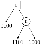
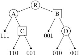
Example 2. Consider the DAGs in Figure 1, where circle and square nodes represent AND-nodes and OR-nodes, respectively. On the left, the lattice is the set of Boolean vectors of length 4 (denoted as words), with bitwise AND and bitwise OR as meet and join, respectively. One can easily verify that v(r) = 1100. On the right, the lattice is the set of Boolean vectors of length 3, and v(R) = 001.

1101 1000

110 001

010 001

Figure 1: Two AND-OR DAGs with partially ordered values.

3.1 Example Applications

Many important problems are in fact AND-OR DAG evaluation in disguise. The simplest one is Boolean circuit evaluation. Here AND- and OR-nodes model AND and OR gates, the lattice is the Boolean algebra (i.e. V = {0, 1} with 0 ⪯ 1 and logical conjunction and disjunction as meet and join), and the evaluation function encodes the inputs of the circuit.

Solving a game with complete information typically involves computing the minimax value of a game tree, which can be regarded as evaluating an AND-OR DAG: AND- and OR-nodes are respectively choice nodes of player MIN and of player MAX, the lattice is (V,≤,min,max) with V a totally ordered set such as Z or R, and the evaluation function gives the value of terminal nodes, or a heuristic value if the search is cut at some depth. Then the root value is the minimax value of the game.

In games with incomplete information, nontrivial lattices come into play. For example, [Ginsberg, 2001] shows that computing the maxmin value of a player amounts to evaluate the game DAG with the lattice (22S ,⪯, ⊓, ∪), where S is a finite set and f ⊓ g = {α ∩ β | α ∈ f, β ∈ g} for any f, g ∈ 22S (i.e. f and g are sets of subsets of S). We will discuss more about this in Section 6.

4 Alpha-Beta Pruning Under Partial Order

Most of the literature on alpha-beta pruning concerns only totally ordered values, such as real numbers. Since AND-OR DAGs with partially ordered values are useful to model richer problems, [Dasgupta et al., 1996] proposed alpha-beta pruning in this new setting for multi-criteria game. [Ginsberg and Jaffray, 2002] gave the first thorough study on this subject, and proved in particular that deep pruning is sound for rational players if and only if the set of values is a distributive lattice. [Loddo and Saiu, 2010] showed that deep pruning is sound for tropical algebras if rationality is relaxed.

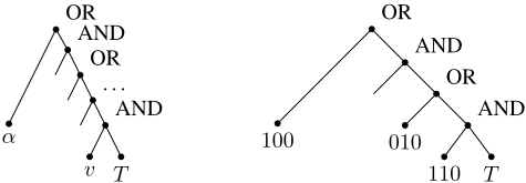
The form of deep α pruning considered by [Ginsberg and Jaffray, 2002] is given in Figure 2 (left). If v ⪯ α, then the subtree T can be deeply pruned. To show why this definition of deep pruning does not capture every cut an alpha-beta search should perform when values are partially ordered, consider Figure 2 (right). The lattice is again the set of Boolean vectors of length 3, with bitwise AND and bitwise OR as meet and join, respectively. When an alpha-beta search algorithm descends to the bottommost AND-node, the value of α would be 110, which is the join of the value of an already explored child of two ancestor OR-nodes. We would like the algorithm

Algorithm 1: Alpha-beta search

1 def AlphaBeta(node n, α, β): 2 I = h(n, α, β) 3 v ← I 4 determine the successor nodes n1, . . . , nb of n 5 for i in {1, . . . , b}: 6 if n is an OR-node: 7 α ← α ∨ v 8 else: 9 β ← β ∧ v 10 if α ⪰ β: 11 break 12 vchild ← AlphaBeta(ni, α, β) 13 if n is an OR-node: 14 v ← v ∨ vchild 15 else: 16 v ← v ∧ vchild 17 return v

to prune subtree T since the value of its parent node cannot be better than the current value of α (due to the sibling of T). However, deep pruning, as it is defined in the literature such as [Ginsberg and Jaffray, 2002], does not apply since the value of α does not come from a child of one single ancestor node. Note that this phenomenon is specific to lattices that are not totally ordered, since otherwise the meet or join (i.e. min or max) of two values is always one of them, hence deep pruning captures any pruning in a standard alpha-beta search.

Another question not formally addressed in the literature is the initialisation of node values. In standard alpha-beta search, one typically initialises the value of an OR-node (respectively AND-node) to be α (respectively β) [Knuth and Moore, 1975] or -∞ (respectively +∞) [Marsland, 1986] (note that -∞ and +∞ translate to ⊥ and ⊤ in our context). However, one may have access to a heuristic evaluation of nodes, typically by evaluating a relaxed version of the problem which is easier to solve. For instance, a player can do no better in a game with incomplete information than in the same game but with complete information. The latter being much easier to solve, the value obtained can be used as a heuristic in the original game with incomplete information. Ideally, initialising values with an accurate heuristic should accelerate the search by finding cuts earlier.

In order to fill these two gaps in the literature, we first formalise alpha-beta search under partial order with initialisation function in Algorithm 1. We denote by h the initialisation function. In general, its value depends on the current α and β, so we define it to yield a value h(n, α, β) for any node n and bounds α and β. Note that since non-trivial initial value can be used for a node n (Line 3), a cut may happen even before the first child of n is explored, hence we update α and β (Lines 7 and 9) and determine whether there is a cut (Line 10) at the beginning of the main loop. This is otherwise the same algorithm as in the literature (for instance, [Marsland, 1986]).

It can be seen that Algorithm 1 will perform the wished pruning in the example in Figure 2 (right). By mimicking the proof by [Knuth and Moore, 1975], we prove that such pruning is indeed sound, thereby extending the result by [Ginsberg and Jaffray, 2002] to its full form, provided that the initialisation function h satisfies a certain admissibility condition:

Definition 3. A heuristic function h is said to be admissible for G and V if for any node n in G and any α, β ∈ V ,

h(n, α, β) = v(n) if n is a leaf node; ⪰ v(n) ∧ β if n is an AND-node; ⪯ v(n) ∨α if n is an OR-node.

Note that this condition is satisfied for the initialisation values usually used in the literature, such as α or -∞ for ORnodes (and β or +∞ for AND-nodes). It is also satisfied when h(n, α, β) overestimates v(n) for internal AND-nodes and underestimates it for internal OR-nodes.

We denote the value returned by Algorithm 1 with input n, α, β by f(n, α, β). The correctness of Algorithm 1 is a consequence of the following central result.

Proposition 1. If h is an admissible heuristic function for G and V , then for any node n of G and any α, β ∈ V , we have β ∧ (α ∨ f (n, α, β)) = β ∧ (α ∨ v(n)).

Intuitively, Proposition 1 states that the value returned by Algorithm 1 is the exact value of n up to a factor of α and β. So even for partially ordered values, alpha-beta search can be interpreted as search with a pruning window.

Now it follows that Algorithm 1 is correct in the sense that if we use a lower and an upper bound as the initial search window at a node, we can recover its exact value using the returned value of the algorithm.

Corollary 1. If h is admissible for G and V , then for any node n of G and any v, v ∈ V satisfying v ⪯ v(n) ⪯ v, we have v(n) = v ∧ (v ∨ f(n, v, v)). In particular, v(n) = f (n, ⊥, ⊤).

Proof. Plug α = v and β = v into the equality in Proposition 1, and use the fact that v ∨ v(n) = v(n) = v ∧ v(n).

Importantly, contrary to the case of totally ordered values, it is not true in general that the stronger equality v(n) = f(n, v, v) holds, as the example in Figure 1 (left) shows. Let h(r, ·, ·) = ⊥ = 0000 and h(n, ·, ·) = ⊤ = 1111, so that h is admissible. Recall that v(r) = 1100. For v = 1000 and v = 1110, indeed v ⪯ v(r) ⪯ v. However, f(r, v, v) = 1101 ̸= v(r) since an α-cut happens in the call on n (Line 10) after examining its first child, since at this point α = β = 1100. However, since α = v and β = v yield no constraint on the fourth component of the values, we still have v(r) = v ∧ (v ∨ f(r, v, v)), as stated in Corollary 1.

5 Alpha-Beta Duo Algorithm

We now come to the main contribution of our work, namely a caching scheme for reusing previously computed values in an alpha-beta search for partially ordered values. The trouble of standard alpha-beta search is that the returned value is equal to the exact value only up to a factor of α and β. It is therefore a nontrivial question how to reuse a previously computed value, since subsequent revisits of a node may come with different search windows.

In alpha-beta search with cache for totally ordered values (for instance [Marsland, 1986]), one can exploit the fact that with usual value initialisation, the value f(n, α, β) satisfies f (n, α, β) < β ⇒ v(n) ≤ f (n, α, β) and f (n, α, β) > α ⇒ v(n) ≥ f(n, α, β). In particular, if α < f(n, α, β) < β, then f(n, α, β) = v(n). Hence by comparing f(n, α, β) to α and β, one can determine whether it is exact, a lower, or an upper bound, and store it in the cache with an appropriate flag.

However, this does not hold in general for partially ordered values, as shown on Figure 1 (right). For α = 010 and β = 110, a β-cut happens after evaluating the first child of C, and an α-cut after evaluating the first child of D. Hence, the algorithm returns 010 for R, which is neither a lower nor an upper bound of the exact value 001. In fact, these two values are incomparable in the lattice. If R is an internal node in a DAG, then caching this returned value 010 may cause an evaluation error when the algorithm revisits R.

To tackle this difficulty, we propose a new algorithm named 'alpha-beta duo', which computes a pair of values for all nodes instead of one single value. The algorithm is presented in Algorithm 2, where Cache refers to a transposition table the entries of which are pairs of values indexed by nodes of G, and (h, h) refers to a pair of initialisation functions for which we assume the following property.

Definition 4. A pair (h, h) of initialisation functions is said to be admissible for G and V if for any node n in G, h(n) ⪯ v(n) ⪯ h(n) holds, and in addition, if n is a leaf node, h(n) = h(n) = v(n) holds.

In other words, admissible h and h respectively underestimates and overestimates the value of a node. Note that h and h that assign respectively ⊥ and ⊤ to all internal nodes form an admissible pair, which can always be used if one does not have better heuristic functions.

Alpha-beta duo search works in the following manner:

• First, variables c and c denote respectively the best lower and upper bound of v(n) available to the algorithm before this call. If n has already been visited, then c and c are retrieved from the cache. Otherwise, they are given by the initialisation functions h and h. If c = c, (c, c) is returned immediately.
• Otherwise, by symmetry consider the case when n is an OR-node. During the main loop, v and v are respectively the cumulative lower and upper bound of v(n) (notice that they are both initialised to ⊥ for an OR-node). If a cut ever happens, it means not all children of n have been evaluated, hence v is not a valid upper bound of v(n). Then we take v to be c, the best upper bound previously known. On the other hand, v, which is the join of lower

1 def AlphaBetaDuo(node n, α, β): 2 if there is an entry for n in the cache: 3 (c, c) ← Cache(n) 4 else: 5 (c, c) ← (h(n), h(n)) 6 if c = c: 7 return (c, c) 8 α←α∨ c 9 β ← β ∧ c 10 if n is an OR-node: 11 (v, v) ← (⊥, ⊥) 12 else: 13 (v, v) ← (⊤, ⊤) 14 determine the children n1, . . . , nb of n 15 for i in {1, . . . , b}: 16 if α ⪰ β: 17 if n is an OR-node: 18 v = c 19 else: 20 v = c 21 break 22 v′ , v′ ← AlphaBetaDuo(ni, α, β) 23 if n is an OR-node: 24 v ← v ∨ v′ 25 v ← v ∨ v′ 26 α ← α ∨ v′ 27 else: 28 v ← v ∧ v′ 29 v ← v ∧ v′ 30 β ← β ∧ v′ 31 v ← v ∨ c 32 v ← v ∧ c 33 store (v, v) in the cache under an entry for n 34 return (v, v)

bounds of children of n that have been evaluated, is a valid lower bound so we keep it.

• Finally, after the main loop, v and v are the lower and upper bounds of v(n) computed by the current call. Hence they are combined with the previously known bounds c and c to yield to best currently known bounds on v(n) and they are cached.

We now prove that alpha-beta duo is correct. For this, we first need the following notion.

Definition 5. A cache Cache is said to be coherent for G and V if for any node n in G, if there is an entry for n in the cache, then Cache(n) = (c, c) where c ⪯ v(n) ⪯ c, and in addition, if n is a leaf node, then c(n) = c(n) = v(n).

Obviously, an empty cache is coherent for any G and V . In the following, we denote the pair of values returned by Algorithm 2 with input n, α, β by (f(n, α, β), f(n, α, β)). We first show that if the cache is initially coherent, then it remains coherent after the execution, and that any interval stored in it cannot become looser.

Proposition 2. If (h, h) is admissible and Cache is initially coherent for G and V , then for any node n in G and any α, β ∈ V , we have f(n, α, β) ⪯ v(n) ⪯ f(n, α, β). Moreover, if there is an entry (c, c) in the cache for n before the call, then c ⪯ f(n, α, β) and f(n, α, β) ⪯ c.

We can now prove results parallel to those in Section 4.

Proposition 3. If (h, h) is admissible and Cache is initially coherent for G and V , then for any node n in G and any α, β ∈ V we have β∧(α∨f (n, α, β)) = β∧(α∨f (n, α, β)).

Corollary 2. If (h, h) is admissible and Cache is initially coherent for G and V , then for any node n in G and any v, v ∈ V satisfying v ⪯ v(n) ⪯ v, we have v(n) = v ∧ (v∨f(n, v, v)) = v∧ (v∨f(n, v, v)). In particular, v(n) = f (n, ⊥, ⊤) = f (n, ⊥, ⊤).

These inequalities are in fact equalities since from Proposition 3 we have v∧ (v∨f (n, v, v)) = v∧ (v∨f (n, v, v)).

6 Experiments

To assess the efficiency of alpha-beta duo (hereafter 'ABD'), we ran experiments comparing it to three other algorithms:

• alpha-beta without cache (Algorithm 1, 'AB' for short);
• an alpha-beta search which only caches the value computed for a node if no cut is found during the search in the subtree rooted at this node (hereafter 'ABC');
• a minimax search algorithmwithout alpha-beta pruning, but with a cache (hereafter 'MMC').

The code of ABD was slightly optimized by refining the values computed on Lines 31 and 32 with the corresponding bounds of all fully explored children. It is easy to show that this preserves the correctness of the algorithm.

For all experiments, we measured the number of nodes of the DAG visited at least once, the total number of node visits (equivalently, the total number of recursive calls), and the time taken for solving the problem. Intuitively, we expect ABD to be better than ABC, ABC to be better than MMC (because MMC does not use alpha-beta pruning), and MMC to be better than AB (because the latter does not cache its results and hence, recomputes several times for the same node).

We used two synthetic sets of benchmarks. The first (hereafter 'random') consists of random DAGs of the same kind as the one in Figure 1. Random DAGs with parameters d (depth), b (branching factor), and v (number of variables) are generated in the following manner:

• d layers 0, 1, . . . , d - 1 are built: layer i consists of 3min(i, 3d 2 -i) nodes (which yields diamond-shapes DAGs);
• from each node n, a set of b nodes is randomly chosen from nodes in the next layer to be C(n);
• each internal node is labelled AND or OR at random;
• the value of each terminal node is a uniformly drawn subset of {1, . . . , v}, or equivalently a random Boolean vector of length v.

We also consider strictly alternating DAGs, in which all nodes in layer i are OR-nodes (respectively AND-nodes) if i is even (respectively odd). In particular, the root is an OR-node.

The second set of benchmarks consists of a simplified version of the card game Bridge that we call 'racing'. There are two players, MIN and MAX. Each has a hand of h cards drawn uniformly from the deck {1, . . . , d} where d ≥ 2h. Players only see their own hand. MIN begins the game. During each trick, the player who begins plays a card from her hand, the other sees it and plays a card in turn. The player who played the highest card wins this trick and starts the next one. No new card is ever drawn from the deck. The game ends when the players have no more cards or when one has won in total g tricks. MAX wins if she is the first one to reach g tricks. For the benchmark, each instance with parameter h, d, and g consists of a randomly drawn hand with h cards for MAX and a randomly drawn card that is supposed to be played by MIN during the first trick. Notice that when d > 2h, each player has incomplete information. We use evaluation of AND-OR DAGs to compute optimal strategies for MAX against the best defence adversary model defined in [Frank and Basin, 1998].

In games with incomplete information where S is the set of all possible hidden configurations, [Frank and Basin, 1998; Frank and Basin, 2001] define the maxmin value of player MAX to be the set of all subsets S′ of S such that there is a uniform strategy winning in any configuration of S′ . [Ginsberg, 2001] shows that computing this value amounts to evaluate the game DAG with the lattice (22S ,⪯, ⊓, ∪). Intuitively, using ∪ at OR-nodes models the fact that player MAX can choose any child as her strategy, and ⊓ at AND-nodes models the fact that a strategy must be robust to all adversarial strategies, hence a strategy wins in s ∈ S if and only if it wins in s whatever action her opponent chooses.

In the same setting of games with incomplete information, one can also be interested in non-uniform strategies which allow player MAX's actions to depend on the hidden information. This can be useful for computing heuristic values of for the game with incomplete information. It can be seen that the set of all configurations for which there is a non-uniform winning strategy can be computed as the value of the game DAG with the lattice (2S , ⊆, ∩, ∪).

Hence, for both benchmarks, we consider the two lattices (22S , ⊓, ∪) and (2S , ∩, ∪). In 'random', S = {1, . . . , v}, while in 'racing' S is the set of all possible hands of player MIN.

For space reasons, we only give the most representative results, in terms of computation time. For each parameter setting and each algorithm, we averaged over 10 runs. Figure 3 shows two examples where, as can be expected, it is more efficient to cache bounds, even more to perform cuts, and still more to compute and store two bounds per node. On the top plot, the gain of using ABD is exponential: with the branching factor increasing, ABD gets a better advantage of computing and caching two bounds. On the bottom plot, ABC and AB (not represented) are exponentially worse, and ABD is better than MMC when the branching factor is high.

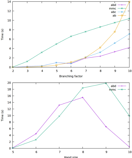
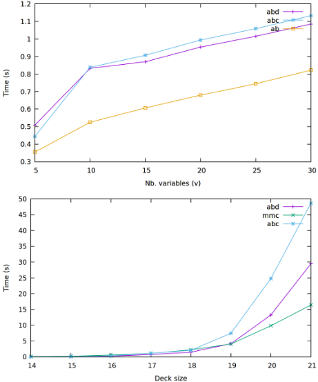
Now Figure 4 shows two examples where it turns out that it is not always better to use alpha-beta pruning with cache.

On the top plot, not caching results at all turns out to be better: the overhead due to the additional operations from the lattice 22S (which are necessary to maintain the cache) seems to compensate the advantage of ABC or ABD in terms of number of visited nodes and recursive calls (the curves are reversed for this metrics, not shown here). On the bottom plot, it turns out that sometimes alpha-beta pruning even degrades performance. Again, this is due to the overhead of manipulating values from a large lattice (for a fixed hand size, the lattice grows exponentially with the deck size).

To complete these results, let us mention that in most experiments, the numbers of nodes explored and visited by each method are ordered as expected, with ratios varying from linear to exponential. In particular, for these metrics, ABD is most of the time better, and often much better, than the other three algorithms.

Summarising, ABD seems to provide a real gain in (brute) performance for DAGs with high branching factors. Contrastingly, when ∧ and ∨ from the lattice are too expensive to compute (as is the case in some large lattices), it may sometimes be better not to use cache and alpha-beta pruning together, due to the overhead to maintain the coherence of the cache.

7 Conclusion

We investigated alpha-beta search for AND-OR DAGs with values from a lattice, which has direct applications such as solving games with incomplete information. We have extended previous formal analyses, in particular to the use of heuristic as initialisation functions. Then we have proposed a new algorithm named 'alpha-beta duo', which caches both a lower and an upper bound of the value of each visited node, and we have formally proved its correctness. Experiments show that it is more efficient than other algorithms in terms of number of visited nodes and recursive calls. As for time efficiency, alpha-beta duo turns out to be more efficient than other algorithms for DAGs with large branching factors and reasonably-sized lattices. As an interesting conclusion, our experiments also put forth that in other cases, it may be better not to use a cache with alpha-beta pruning.

Our future work includes algorithmic optimisations for alpha-beta search with cache applied to games with incomplete information. We will also investigate the use of efficient knowledge representations [Bienvenu et al., 2010; Niveau and Zanuttini, 2016] to accelerate lattice operations in such context. Another perspective is to apply our work to games with multiple criteria instead of scalar outcomes.