
New Bounds and Constraint Programming Models for the Weighted Vertex Coloring Problem
Proceedings of the Thirty-Second International Joint Conference on Artificial Intelligence. Main Track. Pages 1927-1934.
https://doi.org/10.24963/ijcai.2023/214
Keywords
- Search: S: Combinatorial search and optimisation
- Constraint Satisfaction and Optimization: CSO: Constraint programming
Abstract
This paper addresses the weighted vertex coloring problem (WVCP) which is an NP-hard variant of the graph coloring problem with various applications.
Given a vertex-weighted graph, the problem consists of partitioning vertices in independent sets (colors) so as to minimize the sum of the maximum weights of the colors.
We first present an iterative procedure to reduce the size of WVCP instances and prove new upper bounds on the objective value and the number of colors.
Alternative constraint programming models are then introduced which rely on primal and dual encodings of the problem and use symmetry breaking constraints.
A large number of experiments are conducted on benchmark instances.
We analyze the impact of using specific bounds to reduce the search space and speed up the exact resolution of instances.
New optimality proofs are reported for some benchmark instances.
- [Beldiceanu et al., 2005] Nicolas Beldiceanu, Mats Carls- son, and Jean-Xavier Rampon. Global constraint catalog, 2005.
- [Bessiere et al., 2006] Christian Bessiere, Emmanuel He- brard, Brahim Hnich, Zeynep Kiziltan, and Toby Walsh. Filtering algorithms for the nvalueconstraint. Constraints, 11(4):271-293, 2006.
- [Boudhar and Finke, 2000] Mourad Boudhar and Gerd Finke. Scheduling on a batch machine with job com- patibilities. JORBEL-Belgian Journal of Operations Research, Statistics, and Computer Science, 40(1-2):69- 80, 2000.
- [Cai and Lin, 2016] Shaowei Cai and Jinkun Lin. Fast solv- ing maximum weight clique problem in massive graphs. In In Proceedings of the 25th International Joint Conference on Artificial intelligence, pages 568-574, 2016. IJCAI
- [Cheeseman et al., 1991] Peter Cheeseman, Bob Kanefsky, and William M. Taylor. Where the really hard problems are. In Proceedings of the 12th International Joint Confer- ence on Artificial intelligence -Volume 1, page 331-337, 1991. IJCAI
- [Cornaz and Jost, 2008] Denis Cornaz and Vincent Jost. A one-to-one correspondence between colorings and stable sets. Operations Research Letters, 36(6):673-676, 2008.
- [Cornaz et al., 2017] Denis Cornaz, Fabio Furini, and Enrico Malaguti. Solving vertex coloring problems as maximum weight stable set problems. Discrete Applied Mathematics, 217:151-162, 2017.
- [Demange et al., 2007] Marc Demange, D de Werra, Jérôme Monnot, and V Th Paschos. Time slot scheduling of com- patible jobs. Journal of Scheduling, 10(2):111-127, 2007.
- [Frisch et al., 2002] Alan M. Frisch, Brahim Hnich, Zeynep Kiziltan, Ian Miguel, and Toby Walsh. Global constraints for lexicographic orderings. In International Conference on Principles and Practice of Constraint Programming, 2002.
- [Goudet et al., 2022] Olivier Goudet, Cyril Grelier, and Jin- Kao Hao. A deep learning guided memetic framework for graph coloring problems. Knowledge-Based Systems, 258:109986, 2022.
- [Grelier et al., 2022] Cyril Grelier, Olivier Goudet, and Jin- Kao Hao. On monte carlo tree search for weighted ver- tex coloring. In Leslie Pérez Cáceres and Sébastien Verel, editors, Evolutionary Computation in Combinatorial Op- timization, volume 13222 of Lecture Notes in Computer Science, pages 1-16, 2022.
- [Gualandi and Malucelli, 2012] Stefano Gualandi and Fed- erico Malucelli. Exact solution of graph coloring prob- lems via constraint programming and column generation. INFORMS Journal on Computing, 24(1):81-100, 2012.
- [Halldórsson and Shachnai, 2008] Magnús M Halldórsson and Hadas Shachnai. Batch coloring flat graphs and thin. In Scandinavian Workshop on Algorithm Theory, pages 198-209. Springer, 2008.
- [Hébrard and Katsirelos, 2020] Emmanuel Hébrard and George Katsirelos. Constraint and satisfiability reasoning for graph coloring. Journal of Artificial Intelligence Research, 69:33-65, 2020.
- [Hertz and de Werra, 1987] Alain Hertz and Dominique de Werra. Using tabu search techniques for graph color- ing. Computing, 39:345-351, Dec 1987.
- [Liu et al., 2006] Huadong Liu, Micah Beck, and Jian Huang. Dynamic co-scheduling of distributed computa- tion and replication. In Sixth IEEE International Sympo- sium on Cluster Computing and the Grid (CCGRID'06), volume 1, pages 9-pp. IEEE, 2006.
- [Mears et al., 2014] Christopher Mears, Andreas Schutt, Pe- ter J. Stuckey, Guido Tack, Kim Marriott, and Mark Wal- lace. Modelling with option types in minizinc. In Hel- mut Simonis, editor, Integration of AI and OR Techniques in Constraint Programming, pages 88-103, Cham, 2014. Springer International Publishing.
- [Moalic and Gondran, 2018] Laurent Moalic and Alexandre Gondran. Variations on memetic algorithms for graph col- oring problems. Journal of Heuristics, 24(1):1-24, 2018.
- [Nethercote et al., 2007] Nicholas Nethercote, Peter J. Stuckey, Ralph Becket, Sebastian Brand, Gregory J. Duck, and Guido Tack. MiniZinc: Towards a standard CP modelling language. In Christian Bessière, editor, Principles and Practice of Constraint Programming - CP 2007, Lecture Notes in Computer Science, pages 529-543. Springer, 2007.
- [Nogueira et al., 2021] Bruno Nogueira, Eduardo Tavares, and Paulo Maciel. Iterated local search with tabu search for the weighted vertex coloring problem. Computers & Operations Research, 125:105087, Jan 2021.
- [Pachet and Roy, 1999] Franc ¸ois Pachet and Pierre Roy. Au- tomatic generation of music programs. In Joxan Jaffar, ed- itor, In International Conference on Principles and Prac- tice of Constraint Programming, volume 1713 of Lec- ture Notes in Computer Science, pages 331-345. Springer, 1999.
- [Perron and Furnon, 2022] Laurent Perron and Vincent Furnon. Or-tools v9.4. https://developers.google.com/ optimization/, 2022. Accessed: 2023-05-25. Link
- [Prais and Ribeiro, 2000] Marcelo Prais and Celso C. Ribeiro. Reactive grasp: An application to a matrix decomposition problem in tdma traffic assignment. INFORMS Journal on Computing, 12(3):164-176, 2000.
- [Sun et al., 2018] Wen Sun, Jin-Kao Hao, Xiangjing Lai, and Qinghua Wu. Adaptive feasible and infeasible tabu search for weighted vertex coloring. Information Sciences, 466:203-219, Oct 2018.
- [Wang et al., 2020] Shaowei Wang, Yiyuanand Cai, Shiwei Pan, Ximing Li, and Minghao Yin. Reduction and lo- cal search for weighted graph coloring problem. In The Thirty-Fourth AAAI Conference on Artificial Intelligence, AAAI 2020, New York, NY, USA, February 7-12, 2020, pages 2433-2441, 2020.
References were extracted automatically from the PDF and may contain errors.
Full text extracted automatically from the PDF; figures, tables and equations may differ. The PDF is the version of record.
1 Introduction
Given a vertex-weighted graph, the weighted vertex coloring problem (WVCP) consists of partitioning vertices into independent sets (colors) so as to minimize the sum of the maximum weights of the colors. This problem has applications in different domains ranging from metropolitan area network design [Halld´orsson and Shachnai, 2008] and batch scheduling in distributed computing [Liu et al., 2006] to traffic assignment in telecommunications [Prais and Ribeiro, 2000].
Formally, a WVCP instance P = (G,w) is defined by an undirected graph G = (V, E) with vertex set V and edge set E and a function w : V ↦→ N∗ assigning a strictly positive weight w(v) to each vertex v. A (legal) coloring of P is a partition {V1, . . . , Vk} of V into k independent sets of vertices, that is, no pair of vertices in each color Vi is connected in G. The objective is to find a coloring S = {V1, . . . , Vk} whose score f(S) = ∑ki=1 maxv∈Vi w(v) is minimum.
WVCP generalizes the graph coloring problem (GCP) which is NP-hard and consists in determining the chromatic number χG of a graph G, i.e., the minimum size of its colorings. Indeed GCP is the class of WVCP instances whose vertex weights are all equal. Therefore WVCP is also NP-hard.
Various complexity and approximability results have been established for specific classes of WVCP (see e.g. [Boudhar and Finke, 2000; Demange et al., 2007]). New exact methods have been proposed more recently, notably [Cornaz et al., 2017]) which is effective for dense instances, as well as powerful metaheuristics [Wang et al., 2020; Nogueira et al., 2021; Grelier et al., 2022] which have produced new upper bounds for medium and large instances of all types. Constraint Programming (CP) and hybrid CP methods have also been proposed for the graph coloring problem (e.g. [Gualandi and Malucelli, 2012; H´ebrard and Katsirelos, 2020]) but not extended to WVCP to the best of our knowledge.
In this paper, we propose new vertex reduction rules, upper bounds and CP models for WVCP. Building on the work of [Wang et al., 2020], we first present two vertex reduction rules and an iterative procedure to reduce instance size (Section 2). We then establish new upper bounds on the score and number of colors based on the chromatic numbers of the subgraphs induced by the different weight values of an instance (Section 3). Next, we present three CP models for WVCP: a primal model enforcing solution compactness using a dedicated global constraint, a dual model based on a reduction of WVCP to the maximum weighted stable set problem following [Cornaz et al., 2017], and a joint model (Section 4). Lastly, we report experimental results on the CP models and study the impact of pre-computed bounds. The results show that our approach is competitive across a wide variety of benchmark instances (Section 5). The reader is referred to the supplementary material (https: //github.com/Cyril-Grelier/gc wvcp cp) for proofs, complete experimental results, and source code.
2 Vertex Reduction Procedure
This section presents an iterative vertex reduction procedure for WVCP using two rules. We shall denote by N(v) = {u ∈ V | {u, v} ∈ E} the neighborhood of vertex v in G = (V, E), and ∆ = maxv∈V |N(v)| the degree of G. A clique C of G is a subset of V whose vertices are pairwise adjacent.
2.1 Reduction Rules
[Wang et al., 2020] proposed a reduction rule (R0) consisting in comparing the weight of a vertex u with the weights of the vertices of a given clique C of the graph G, such that u /∈ C. We propose an improvement R1 to this rule, which takes into
Algorithm 1 POSICLIQUE
- 1: Input: WVCP instance P = (G,w), vertex u ∈ V and clique C = {c1, . . . , c|C|} s.t. w(ci) ≥ w(cj) (1 ≤ i < j ≤ |C|).
- 2: Output: d ∈ N∗
- 3: d ← |N(u)| +1 ; lC ← |C| - 1
- 4: for i from 0 to lC do
- 5: if c|C|-i ∈ N(u) and |C| - i ≥ d then
- 6: d ← d - 1
- 7: return d
account the fact that u may have neighbors in C using the POSICLIQUE procedure.
Rule 1. Let P = (G,w) be a WVCP instance with G = (V,E), C a clique of G, u ∈ V \ C, and d = POSICLIQUE(u,C). If d ≤ |C| and w(u) ≤ w(cd), the optimal score of P is unchanged after removing u from G.
Proof. See supplementary material.
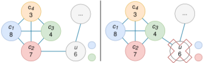
This first rule (R1) is equivalent to the rule R0 when N(u) ∩ C = ∅. In this case, d = |N(u)| + 1 and u is removed if d ≤ |C| and w(u) ≤ w(cd). However, our rule is stronger when N(u) ∩ C ̸= ∅ since the value d returned by POSICLIQUE may be lower than |N(u)| + 1 which improves the chance of a successful check w(u) ≤ w(cd) due the weight-based decreasing order assumed on the vertices of cliques. Note that the worst-case time complexity of the rule is O(∆2 ).
Figure 1 sketches two graphs including a clique C = {c1, c2, c3, c4} and a vertex u of weight 6 to illustrate the evaluation of the rule. In both cases, |N(u)| = 2. On the left, c2 ∈ N(u). Thus, given u and C as inputs, POSICLIQUE returns d = 3 and u cannot be deleted since it may have to take the same color as c3 in the worst case and its weight is greater than w(c3) = 4. On the right, c3 ∈ N(u). In this case, POSICLIQUE returns d = 2 and u can be removed since it can take the blue or red color, and in either case, there is no impact on the WVCP score because its weight of 6 is lower than w(c1) = 8 and w(c2) = 7. Note that the rule R0 does not allow to remove u in these two scenarios since w(u) is strictly greater than w(c|N(u)|+1) = 4.
Our second reduction rule (R2) is an adaptation of the second reduction operator originally proposed by [Cheeseman et al., 1991] for the k-coloring problem. Its worst-case time complexity is O(∆2 ).
Rule 2. Given a WVCP instance P = (G,w) with G = (V,E) and two vertices u, v ∈ V such that N(u) ⊂ N(v) and w(u) ≤ w(v) then the optimal score of P is unchanged after removing vertex u from G.
Proof. See supplementary material.
2.2 MaximumWeighted Cliques Extraction and Iterative Reduction
R1 considers the deletion of a vertex relatively to a single clique. We propose to widen its scope by applying it to different cliques of G = (V, E). Ideally, each clique C should have maximum weight ∑c∈C w(c). However, finding a clique of maximum weight in a graph is NP-hard so we rely on a fast heuristic to perform this task, namely, the FastWClq algorithm [Cai and Lin, 2016]. FastWClq iteratively builds a clique with greedy moves using any vertex as a starting point. To keep run time acceptable while aiming for diversity across cliques, we compute |V | cliques by generating a single clique per vertex v ∈ V using v as the starting point for FastWClq. This procedure is O(|V |3 ).
Once the cliques generated, the two reduction rules are applied to each vertex by increasing order of weights. Each time a vertex is deleted, it is stored in a list L and the graph G and the set of cliques are updated to take the deletion into account. The process is repeated until no vertex can be removed. This iterative procedure is O(∆2 |V |3 ). When a solution is found for the instance P ′ = (G′ , w) produced by the reduction procedure, it is possible to obtain a solution of the same score for the original instance P = (G, w) by coloring each vertex of the list L with a greedy algorithm in the reverse order of arrival in L.
3 Upper Bounds on Score and Number of Colors
Theorem 1 introduces new upper bounds on the score and number of colors to solve a WVCP to optimality. These bounds are based on the chromatic numbers of the subgraphs induced by each weight value. We denote by W = {w(v) | v ∈ V } the set of weight values used in G, Gw = (Vw,Ew) the subgraph of G induced by weight w where Vw = {v ∈ V | w(v) = w} and Ew = {{u, v} ∈ E | u, v ∈ Vw}, and χGw the chromatic number of Gw.
Theorem 1. Given a WVCP instance P = (G, w) with G = (V, E) and an optimal solution S∗ = {V1, . . . , Vk} of P corresponding to a partition of V into k non-empty independent sets, then k ≤ ∑w∈W χGw and f (S∗ ) ≤ ∑w∈W w × χGw .
Proof. See supplementary material.
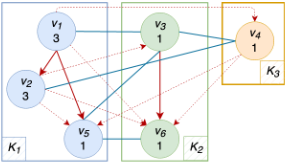
Consider the WVCP instance shown in Figure 2. The upper bounds derived from Theorem 1 on the number of colors and the score are respectively equal to 3 = χ3 + χ1 = 1 + 2 and 5. Both bounds are exact in this case and the solution shown is optimal. Computing the upper bounds involves solving |W| GCP sub-problems to obtain the chromatic numbers χGw (w ∈ W). Since GCP is NP-hard, the chromatic numbers may be upper-bounded using heuristics for GCP such as TabuCol [Hertz and de Werra, 1987] (see Section 5.2).
4 Constraint ProgrammingModels
This section introduces three alternative CP models for WVCP called primal, dual, and joint. We shall use the following notations. Given a set S, [S] denotes the range {1, . . . , |S|}. For a function f : X ↦→ Y and X′ ⊆ X, f(X′ ) denotes the image of X′ by f and f -1 : Y ↦→ 2X the function defined by f -1 (y) = {x ∈ X|f(x) = y}. For a vertex v of a graph G, N(v), ∆(v) and ∆(G) denote respectively the set of neighbours of v, its degree and the maximum vertex degree in G.
Let κ ∈ N∗ and P be a WVCP instance of graph G = (V, E) and weight function w, Pκ denotes the problem of determining the existence of a solution to P that uses a number of colors smaller than or equal to κ. Given a pair (P, κ), each model searches for an optimal solution to Pκ. i.e. a solution s to Pκ whose score f(s) is the lowest among all solutions to Pκ. A model may therefore be instantiated with κ = |V | to solve P optimally or with any known upper bound κ < |V | on the number of colors. Note that an optimal solution for Pκ is not necessarily optimal for P. Consider the instance P of Figure 2. The optimal score for P3 is the score of the solution shown and equal to 5 whereas the optimal score for P2 is 6.
The CP models require a total ordering ≥w over V which is consistent with the descending order of weights (u ≥w v → w(u) ≥ w(v) for u, v ∈ V ). We shall say that vertex u dominates vertex v if u ≥w v. The dominance ordering may be freely chosen and it is encoded by a consistent indexing of vertices over [V ] (vi ≥w vj ↔ i ≤ j for i, j ∈ [V ]). 1 Solutions to Pκ are thus modeled as maps s : [V ] ↦→ K where K = {1, . . . , κ} is the range of colors. In order to break symmetries induced by color permutation, the computation is restricted to d-sorted solutions also called d-solutions. A solution is d-sorted if non-empty colors start from rank 1 and are sorted consistently with the ordering ≥w of their dominant vertices. Formally, s : [V ] ↦→K is d-sorted if s([V ]) = [s([V ])] and min(s-1 (j)) < min(s-1 (k)) for 1 ≤ j < k ≤ |s([V ])|. Clearly, the set of solutions to Pκ is in one-to-one correspondence with the set of d-solutions which we shall denote by SPκ .
The primal model of Pκ represents vertex coloring decisions as variables and uses symmetry breaking constraints to compute optimal and compact d-sorted solutions. The dual model is based on a reduction of WVCP to the maximum weighted stable set problem which turns the complement of G into a directed graph using the chosen ordering ≥w [Cornaz et al., 2017]. Dual variables represent decisions to keep or remove arcs in this digraph so as to construct pairwise vertexdisjoint simplicial stars. The simplicial stars of a dual solution map one-to-one with the colors of size ≥ 2 in the primal solution, the center of a star being the dominant vertex in the corresponding color. A dual solution is scored by summing the weights of the target nodes in the simplicial stars. The sum of the dual and primal scores of a solution is therefore equal to the sum of the weights over all vertices. The joint model is essentially a combination of the primal and dual models using channeling constraints. Figure 2 illustrates the primal and dual representations of a d-solution.
1 The dominant vertex vi in a set of vertices {vi1 , . . . , vin } is thus identified by i = min{i1, . . . , in}.
4.1 Primal Model
The primal model supports variability in the number of colors used across solutions and includes symmetry breaking constraints. To allow for the possibility that some colors of K may have no vertices in a solution, G is extended with virtual vertices. Specifically, a disconnected vertex uk of weight 0 is introduced for each color k ∈ K and systematically assigned to k in any solution. The weight function w is extended accordingly to cover the whole set of vertices U = V ∪{uk|k ∈ K} and so is dominance ordering ≥w. The latter is encoded by a consistent indexing of vertices over [U] (vi ≥w vj ↔ i ≤ j for i, j ∈ [U]).
The model is given by constraints (P1-P10) and uses global constraints INT SET CHANNEL and STRICTLY INCREASING [Beldiceanu et al., 2005]. (P1) models the WVCP score to minimize with integer variable xo which is lower-bounded by the maximum vertex weight and upper-bounded by the sum of the weights (or any given bounds). (P2) associates each vertex vi ∈ U with an integer variable xUi representing its coloring in a solution. Each color k ∈ K is associated with a set variable xKk representing its set of vertices (P3) and an integer variable xDk representing its dominant vertex (P4).
minimize xo s.t.
(P5) links vertex and color variables through a channeling constraint involving auxiliary boolean variables that reify domain membership (xUi = k ↔ i ∈ xKk for all vi ∈ U, k ∈ K). (P6) enforces a one-to-one mapping between virtual vertices and colors thereby ensuring the existence of a dominant vertex for each color. (P7) models the coloring constraints induced by G. (P8) defines the dominant vertex (possibly virtual) of each color. (P9) models the scoring function as the sum of the weights of the dominant vertices using element constraints. Note that empty colors get cancelled out in this sum. Lastly, (P10) enforces the dominance ordering on colors (xDk-1 < xDk for 2 ≤ k ≤ |K|). No lexicographic ordering constraint [Frisch et al., 2002] is needed here due to the indexing of vertices using ≥w.
We now formalize a compactness property for d-solutions and show that every WVCP instance (G,w) has optimal dsolutions which are compact. Such solutions are computable with a maximum of ∆(G)+1 colors. We then propose a global constraint that guarantees solution compactness when it is applied to the neighborhood of each vertex. Informally, a d-solution is compact if the color of any vertex is the lowest in K that is left free by its neighbors. In other words, no vertex may be "left-shifted" to a lower-ranked color without violating coloring constraints. For instance, the d-solution in Figure 2 is compact since neither v3, v4 nor v6 may be leftshifted. If (v3, v4) and (v5, v6) were not part of the graph, then v6 and v4 could be left-shifted to colors K1 and K2 respectively to compact the solution. Solution compactness is defined using a function which computes the lowest possible color for a vertex in a d-solution.
Definition 1. Let Pκ be a satisfiable WVCP instance and µPκ : SPκ × V ↦→ K such that, for all s ∈ SPκ , v ∈ V , µPκ (s, v) = mink=1..∆(v)+1({k | ∀u ∈ N(v) : s(u) ̸= k}). s ∈ SPκ is compact if µPκ (s, v) = s(v) for all v ∈ V .
µPκ clearly exists and is uniquely defined since the neighbors of a vertex v may not use more than ∆(v) colors in the range {1, . . . ,∆(v)+1}. Besides, left-shifting a vertex v using µPκ may only decrease the score of a d-solution s or leave it unchanged. However, the resulting solution may not be dsorted if v was the dominant vertex of an intermediate color k < |s(V )| and the latter gets empty or dominated by the next color after the shift. The resulting solution may also include a greater number of vertices that can be left-shifted compared to the original solution. Theorem 2 shows there actually exists an idempotent function that turns any d-solution into a compact d-solution with no score increase. The proof is based on a recursive algorithm which, given a d-solution, combines vertex left-shifting (µPκ ) with color left-shifting and swap operations to converge towards a compact d-solution.
Theorem 2. Let Pκ be a satisfiable WVCP instance. There exists gPκ : SPκ ↦→ SPκ such that, for all s ∈ SPκ , gPκ (s) is compact, f(gPκ (s)) ≤ f(s) and gPκ (gPκ (s)) = gPκ (s).
An immediate corollary of Theorem 2 is that every satisfiable instance Pκ has an optimal d-solution which is compact. Therefore, every WVCP P has an optimal solution which is a compact and optimal d-solution for Pκ with κ = |V |. By definition of µPκ , no vertex v is colored beyond the first ∆(v)+1 colors in this solution. It follows that the maximum degree of G plus 1 is a safe upper-bound on the number of colors needed to optimally solve P as already proved in [Demange et al., 2007]. Hence Pκ with κ = ∆(G) + 1 has an optimal and compact d-solution which is also optimal for P .
Corollary 1. Let P be a WVCP instance. P∆(G)+1 has an optimal and compact d-solution which is optimal for P .
Thanks to Corollary 1, the primal model may be safely instantiated with ∆(G) + 1 colors and, by definition of µPκ , be tightened with constraints upper-bounding the domain of each vertex variable xUi with∆(vi)+1. We now introduce the global constraint MAX LEFT SHIFT to enforce solution compactness. MAX LEFT SHIFT applies to a vector of n positive integer variables and determines the lowest value in the range {1, . . . , n + 1} that is not assigned to any of these variables.
Definition 2. Let y be an integer domain variable and [x1, . . . , xn] be a vector of positive integer domain variables (n ≥ 0). MAX LEFT SHIFT(y, [x1, . . . , xn]) holds iff y = mink=1..n+1({k | ∀i = 1..n : xi ̸= k}).
Applying MAX LEFT SHIFT in the primal model to the variable of a vertex vi and those of its neighbors as formulated in constraint (P11) clearly amounts to enforcing compactness equation µPκ (s, vi) = s(vi) on any d-solution s. (P11) thus ensures only compact d-solutions may be generated with the primal model. Note that (P11) makes all coloring constraints (P7) redundant by definition of MAX LEFT SHIFT.
We now provide a decomposition of MAX LEFT SHIFT using constraints (M1-M4). The decomposition relies on global constraint NVALUE [Pachet and Roy, 1999; Bessiere et al., 2006] which counts the number of different values assigned to a vector of variables: NVALUE(y, [z1, . . . , zn]) holds iff y = |{zi|i = 1 . . . n}|. Constraint (M1) enforces that y be different from each xi (equivalent to (P7)). (M2) associates to each xi a variable zi ranging over {0, . . . , n + 1}. (M3) either sets zi to xi if the latter is strictly smaller than y or to 0 otherwise. This is achieved by reifying constraint y > xi with an implicit 0/1 variable. (M4) sets y to the number of different values taken in the vector including all variables zi and a ground variable of value 0. Any variable xi strictly greater than y does not contribute to the count (i.e. the value of y) since its variable zi is absorbed by value 0 in the vector. Hence y is the number of different values taken by the variables it is strictly greater than plus 1 (value 0). Since all variables are positive, this number is necessarily the lowest possible value for y (n + 1 in the worst-case).
4.2 Dual Model
The dual model for problem Pκ is a CP adaptation of the MIP model of [Cornaz et al., 2017]. The latter applies to a dual graph based on a reduction of WVCP to the maximum weighted stable set problem [Cornaz and Jost, 2008]. Given a WVCP P = (G, w) and a dominance ordering ≥w, the dual graph is built by turning each edge {vi, vj} of the complement of G such that vi ≥w vj into the arc (vi, vj) of source node vi and target node vj . We denote by # � Ec = {ij | vi, vj ∈ V ∧{vi, vj} /∈ E∧vi ≥w vj} the set of arcs of the dual graph, and T its set of target nodes (nodes with incoming arcs).
The reduction relies on the notion of a simplicial stellar forest. A pair of arcs (ij, ik) is simplicial if an arc exists between j and k in the dual graph. A star (i.e. a set of arcs with the same source node) is simplicial if each pair of arcs in the star is simplicial in the dual graph. A simplicial stellar forest is a set of simplicial stars that span disjoint subsets of nodes. [Cornaz et al., 2017] show that the legal colorings of a WVCP instance map one-to-one with the simplicial stellar forests of its dual graph. Note that singleton colors in a WVCP solution map to the disconnected nodes in the corresponding forest. A simplicial stellar forest is scored by summing the weights of the target nodes of its arcs. This score added to the WVCP score of the corresponding primal solution is therefore equal to the sum of the weights of all the vertices (see Figure 2).
maximize yo s.t.
The dual model is given by constraints (D1-D10). (D1-D6) correspond to the MIP model used to compute simplicial stellar forests. (D1) associates the arcs of # � Ec with 0/1 variables representing the exclusion (yA ij = 0) or inclusion (yA ij = 1) of each arc ij in the forest. (D2) models the score to maximize and (D3) the scoring function. (D4) forbids non-simplicial stars. (D5) forbids the chaining of arcs and (D6) multiple incoming arcs to enforce disjointness and star structure.
Colors are not computed in the MIP model but must be counted and upper-bounded here to solve Pκ. To this effect,
(D7-D10) make color dominants explicit. (D7) defines 0/1 variables indicating if a node vi is the dominant vertex of a color in the corresponding WVCP solution (zV i = 1) or not (zV i = 0). Based on the reduction, a node is dominant iff it is the center of a simplicial star (hence dominating a color of size ≥ 2) or it is disconnected in the forest (hence being the only node in its color). We consider two cases based on whether vi is a target node in the dual graph (D8) or not (D9). (D8) ensures that a target node is dominant iff it is not the target of any arc in the simplicial stellar forest (e.g. v3 and v4 in Figure 2). (D9) ensures that a node which is not a target node in the graph can never be dominated. The top node v1 and each disconnected node in the graph always fall into this category. Since every color has a single dominant, (D10) upper-bounds the number of dominants with κ. Note that, as opposed to the primal model, no symmetry breaking is needed here to handle color permutation, neither is optionality modeling [Mears et al., 2014] to handle unused colors.
4.3 Joint Model
The joint model combines the primal and dual models with constraints (J1-J4). Despite a quadratic space complexity (it encodes the instance graph and its complement), one may expect benefits from the bi-directional propagation, especially for graphs of average density which incur the lowest overhead compared to the other models. (J1-J3) are the core constraints matching the primal and dual solutions. (J1) states that the presence of an arc in the dual solution is a sufficient condition for its two vertices be colored identically. (J2) matches the color dominants in the two representations using a global cardinality contraint and (J3) models the equation linking primal and dual solution scores. (J4) is equivalent to (P11) but considers non-adjacent vertices instead of neighbours to leftshift a vertex. Given a vertex vi and any non-adjacent dominant vertex vj ≥w vi, (J4) enforces that vi is in vj's color or a lower-ranked color if none of its neighbors vh is in vj's color.
minimize xo s.t.
∀vi ∈ V, vj ∈ N(vi) s.t. vj ≥w vi :
5 Experiments
We first introduce the benchmark instances used for experiments and analyse the impact of our reduction procedures on instance size. We then discuss the impact of using precomputed bounds on problem-solving efficiency. Lastly, we compare the results of our CP models with the state-of-the-art.
Benchmark instances. A total of 188 WVCP instances were considered: 30 rxx graphs and 35 pxx graphs from matrix decomposition problems [Prais and Ribeiro, 2000] and 123 graphs coming from the DIMACS and COLOR competitions [Sun et al., 2018]. Due to lack of space, we report detailed results on 12 instances of different sizes, graph densities, and weight and degree distributions. Complete benchmark instances, source code, and results are available in the supplementary material.
Experimental settings. Experiments were performed on an Intel Xeon ES 2630, 2.66 GHz, Broadwell. CP models were programmed using Minizinc [Nethercote et al., 2007] and solved using OR-Tools [Perron and Furnon, 2022]. We used heuristics first-fail combined with domain bisection to solve primal and joint instances and a static heuristics sorting arcs by descending order of weights to solve dual instances. A time limit of 1 hour using a single CPU was set for each run.
5.1 Reduction of Instance Sizes
Table 1 reports the impact of the different reduction rules on the whole set of 188 instances. As for R0 and R1, we precomputed a set of cliques C as discussed in Section 2.1 then applied each rule individually to each pair (v, c) with v ∈ V and c ∈ C (lines R0 and R1). As for R2, we applied the rule to each pair of non-adjacent vertices. (R1 + R2) corresponds to the joint application of the two reduction rules. Lastly Iterative corresponds to the iterative reduction procedure (see Section 2.2) which applies R1 and R2 until no vertex can be removed.
We see that R1 works slightly better than R0 in terms of number of reduced instances (# RI) and average percentage of reduction (%RV) for these reduced instances. Overall, we observe a great improvement due to the iterative procedure. The computational time required to perform the different reductions remains reasonable in average in comparison with rule R0 (see column 7).
We will only consider the reduced instances in the experiments described in the rest of the paper. Note that using the reduced instances allows to greatly improve the results compared to the original ones (see supplementary material).
5.2 Bounds on Number of Colors and Score
Table 2 shows lower and upper bounds on the score and the number of colors required for an optimal solution given by Theorem 1 or coming from previous studies.
Columns 1-4 show the different characteristics of the instances. Column 4 introduces a measure of weight heterogeneity defined by hW = |W| |V | . Column 5 reports the value ∆ + 1 (∆ denotes the maximum vertex degree in the graph)
| #RI | #RV avg | #RV max | %RV avg | %RV max | t(s) avg | |
|---|---|---|---|---|---|---|
| R0 | 82 | 34.2 | 469 | 13.4 | 65 | 2.6 |
| R1 | 84 | 39.5 | 574 | 14.7 | 66.4 | 3.8 |
| R1+R2 | 85 | 41.7 | 596 | 15.4 | 69 | 4.1 |
| Iterative | 85 | 54.3 | 683 | 23.3 | 80.9 | 9.8 |
which is a baseline upper bound on the number of colors required to obtain an optimal solution [Demange et al., 2007]. Column 6 reports a lower bound on the number of colors which corresponds to the maximum size of a clique in G found with the clique extraction procedure applied during the first reduction pre-processing step (see Section 2.2). Column 7 corresponds to the upper bound on the number of colors given by Theorem 1. This bound was obtained by solving |W| GCP sub-problems with decreasing number of colors using the C++ implementation of the TabuCol algorithm [Hertz and de Werra, 1987] proposed in [Moalic and Gondran, 2018] with a limit of 1000 iterations without improvement for each graph k-coloring sub-problem. It does not take more than 0.1 second per instance to compute the global upper bound with this method. This upper bound is written in bold when it is better than the bound ∆ + 1, which happens almost all the time, except for specific instances such as r30 characterized with a high weight heterogeneity hW. Column 8 is a lower bound on the score computed with the method proposed by [Wang et al., 2020] (see Proposition 1) and using the set of maximum weighted cliques computed with the FastWClq algorithm. Column 9 reports the upper bound on the score computed according to Theorem 1.
5.3 Impact of Color and Score Bounds
Table 3 shows the impact on the primal model of the upper bound on the number of colors (see Theorem 1) as well as the impact of introducing simultaneously all the bounds presented in the last section. The impact of the other bounds each taken separately is presented in the supplementary material.
Column 1 is the name of the instance. Column 2 reports the best-known score (BKS) obtained in the literature. Some of these BKS were obtained under specific and relaxed conditions, such as one day of computation in parallel on Graphic Processing Device (GPU) in [Goudet et al., 2022], and are therefore very difficult to reach. When a star is added to this score, it means that it has been proven optimal. Most of these proofs of optimality were obtained with the MIP formulation of [Cornaz et al., 2017] solved during 10h using CPLEX [Nogueira et al., 2021].
A score is written in bold in columns 3-8 when it corresponds to the BKS. When the instance is solved to optimality, a star is added and the time in seconds required to prove optimality is reported. Otherwise "tl" is indicated meaning that the time limit of 1 hour has been reached. The score is underlined if this optimality has never been proved before in the literature.
| colors bounds | score bounds | |||||||
|---|---|---|---|---|---|---|---|---|
| Instance | |V ′ | | density | hW | ∆+1 | lb | ub | lb | ub |
| DSJC125.1g | 125 | 0.1 | 0.04 | 24 | 4 | 14 | 19 | 42 |
| DSJC125.5g | 125 | 0.5 | 0.04 | 76 | 10 | 34 | 42 | 105 |
| DSJC125.9g | 125 | 0.9 | 0.04 | 121 | 32 | 72 | 124 | 220 |
| DSJR500.1 | 244 | 0.03 | 0.08 | 26 | 12 | 26 | 166 | 477 |
| GEOM110 | 87 | 0.11 | 0.11 | 20 | 9 | 20 | 65 | 151 |
| inithx.i.1 | 181 | 0.05 | 0.1 | 169 | 54 | 78 | 569 | 800 |
| le450 15a | 420 | 0.08 | 0.05 | 99 | 15 | 61 | 206 | 628 |
| le450 25b | 345 | 0.08 | 0.06 | 108 | 25 | 73 | 307 | 735 |
| mulsol.i.5 | 104 | 0.23 | 0.18 | 88 | 31 | 58 | 367 | 574 |
| queen10 10 | 100 | 0.59 | 0.19 | 36 | 10 | 36 | 153 | 420 |
| p42 | 135 | 0.12 | 0.46 | 25 | 14 | 25 | 2466 | 8108 |
| r30 | 301 | 0.09 | 0.76 | 35 | 19 | 35 | 9816 | 104285 |
| primal | primal ub color | primal all bounds | |||||
|---|---|---|---|---|---|---|---|
| instance | BKS | score | time(s) | score | time(s) | score | time(s) |
| DSJC125.1g | 23 | 23* | 862 | 23* | 435 | 23* | 451 |
| DSJC125.5gb | 240 | 270 | tl | 270 | tl | 270 | tl |
| DSJC125.5g | 71 | 78 | tl | 78 | tl | 78 | tl |
| DSJC125.9g | 169* | 176 | tl | 176 | tl | 176 | tl |
| DSJR500.1 | 169 | 187 | tl | 177 | tl | 169 | tl |
| GEOM110 | 68* | 69 | tl | 68* | 1893 | 68* | 1729 |
| inithx.i.1 | 569* | 569 | tl | 569 | tl | 569* | 54 |
| le450 15a | 212 | 245 | tl | 234 | tl | 234 | tl |
| le450 25b | 307 | 307 | tl | 307 | tl | 307* | 322 |
| mulsol.i.5 | 367* | 367 | tl | 367 | tl | 367* | 31 |
| queen10 10 | 162 | 170 | tl | 169 | tl | 169 | tl |
| p42 | 2466* | 2480 | tl | 2466 | tl | 2466* | 2908 |
| r30 | 9816* | 9831 | tl | 9831 | tl | 9831 | tl |
| nb bks reached nb optim | 101/188 72/188 | 105/188 75/188 | 107/188 95/188 | ||||
We see that the upper bound on the number of colors (Columns 5-6) deriving from Theorem 1 can significantly reduce the time spent by the solver on each instance, because it reduces the domain of available colors for each vertex.
Columns 7-8 correspond to the results when all the lower and upper bounds presented in Table 2 are simultaneously activated, which allows to increase the number of BKS reached (107 out of 188), as well as the number of optimality proofs (95 out of 188) for the whole set of instances.
5.4 Comparison of CP Models
Table 4 compares the results obtained by the three CP models described in Section 4 (primal, dual and, joint) on the same set of reduced instances, without using pre-computed bounds. Columns 3-4 report the results of the primal model (P1-P10) and Columns 5-6 correspond to the results of the primal model extended with compactness constraints (P11) and decomposed using constraints (M1-M4). When enforcing compactness, the number of instances solved to optimality goes from 72 to 76, indicating that dynamically reducing the color domain of each vertex during the search can be beneficial. Columns 7-8 report the results of the dual model presented in Section 4.2 (D1-D10). We observe that the primal and dual models obtain different results depending on the density of the instance. Unsurprisingly, the primal model is better for instances characterized by a low graph density (in particular it can reach a new optimality proof for instance DSJC125.1.g), while the dual is better for instances with high-density graphs such as DSJC125.9.g. In Columns 9-10, we observe that the joint model coupling the primal and dual models (P1-P10, D1-D10 and J1-J4), performs well on both low and high density instances, as it can take advantage of both models. It solves 100 instances over 188 to optimality, which is the highest number. Moreover, results on some instances such as inithx.i.1, mulsol.i.5 and p42, which go beyond the results obtained by the primal and dual models alone, show that it can benefit from a synergy of the two representations.
| primal | primal + P11 | dual | joint + J4 | ||||||
|---|---|---|---|---|---|---|---|---|---|
| instance | BKS | score | time(s) | score | time(s) | score | time(s) | score | time(s) |
| DSJC125.1g | 23 | 23* | 862 | 23* | 628 | 26 | tl | 24 | tl |
| DSJC125.5g | 71 | 78 | tl | 78 | tl | 84 | tl | 78 | tl |
| DSJC125.9g | 169* | 176 | tl | 176 | tl | 169* | 56 | 169* | 380 |
| DSJR500.1 | 169 | 187 | tl | 173 | tl | 187 | tl | 186 | tl |
| GEOM110 | 68* | 69 | tl | 68* | 53 | 73 | tl | 68* | 741 |
| inithx.i.1 | 569* | 569 | tl | 569 | tl | 569 | tl | 569* | 1923 |
| le450 15a | 212 | 245 | tl | 235 | tl | 250 | tl | - | tl |
| le450 25b | 307 | 307 | tl | 310 | tl | 314 | tl | - | tl |
| mulsol.i.5 | 367* | 367 | tl | 367 | tl | 367 | tl | 367* | 203 |
| queen10 10 | 162 | 170 | tl | 170 | tl | 177 | tl | 172 | tl |
| p42 | 2466* | 2480 | tl | 2480 | tl | 2517 | tl | 2466* | 673 |
| r30 | 9816* | 9831 | tl | 9831 | tl | 9831 | tl | 9831 | tl |
| nb BKS reached nb optim | 101/188 72/188 | 102/188 76/188 | 79/188 68/188 | 112/188 100/188 | |||||
| instance | |V | | BKS | score | time(s) | instance | |V | | BKS | score | time(s) |
|---|---|---|---|---|---|---|---|---|---|
| DSJC125.1gb | 125 | 90 | 90* | 25 | myciel7gb | 191 | 109 | 109* | 69 |
| DSJC125.1g | 125 | 23 | 23* | 11 | myciel7g | 191 | 29 | 29* | 241 |
| DSJR500.1 | 500 | 169 | 169* | 66 | queen9 9g | 81 | 41 | 41* | 509 |
| myciel6gb | 95 | 94 | 94* | 17 | queen10 10g | 100 | 43 | 43* | 820 |
| myciel6g | 95 | 26 | 26* | 17 | le450 25b | 450 | 307 | 307* | 322 |
5.5 NewOptimality Proofs
We launched the primal, dual, and joint models with compactness constraints and using pre-computed bounds on a server with 10 threads and a time limit of 1 hour. Table 5 reports all the new optimality proofs obtained for difficult instances during all our experiments (see supplementary material for complete tables).
6 Conclusion
We proposed an iterative reduction procedure and established new upper bounds on the score and the number of colors needed to optimally solve WVCP. We highlighted their practical value in reducing the search space through experiments carried out on benchmark instances. Three CP models were also investigated together with global constraints to break symmetries. We provided empirical evidence to shed light on their advantages and limits. The results showed that the models are competitive for most of the small- and mediumsize instances, leading in particular to solving some instances to optimality. In our future work, we would like to investigate possible hybridizations of the CP models with metaheuristics based in particular on the proposed compactness algorithm.
Acknowledgements
We are grateful to the reviewers for their feedback. We thank B. Nogueira for sharing his CPLEX code used in [Nogueira et al., 2021] and A. Go¨effon for fruitful exchanges on the reduction rules. We acknowledge support from the Centre R´egional de Calcul Intensif des Pays de la Loire (CCIPL) for hosting experiments.
@inproceedings{ijcai2023p214,
  title     = {New Bounds and Constraint Programming Models for the Weighted Vertex Coloring Problem},
  author    = {Goudet, Olivier and Grelier, Cyril and Lesaint, David},
  booktitle = {Proceedings of the Thirty-Second International Joint Conference on
               Artificial Intelligence, {IJCAI-23}},
  publisher = {International Joint Conferences on Artificial Intelligence Organization},
  editor    = {Edith Elkind},
  pages     = {1927--1934},
  year      = {2023},
  month     = {8},
  note      = {Main Track},
  doi       = {10.24963/ijcai.2023/214},
  url       = {https://doi.org/10.24963/ijcai.2023/214},
}
TY - CPAPER TI - New Bounds and Constraint Programming Models for the Weighted Vertex Coloring Problem AU - Goudet, Olivier AU - Grelier, Cyril AU - Lesaint, David T2 - Proceedings of the Thirty-Second International Joint Conference on Artificial Intelligence, IJCAI-23 PB - International Joint Conferences on Artificial Intelligence Organization PY - 2023 SP - 1927 EP - 1934 DO - 10.24963/ijcai.2023/214 UR - https://doi.org/10.24963/ijcai.2023/214 ER -Copied
Machine-readable versions of this paper, for tools and AI agents:





