
Flaws of Termination and Optimality in ADOPT-based Algorithms
Proceedings of the Thirty-Second International Joint Conference on Artificial Intelligence. Main Track. Pages 1996-2003.
https://doi.org/10.24963/ijcai.2023/222
Keywords
- Constraint Satisfaction and Optimization: CSO: Constraint optimization
- Constraint Satisfaction and Optimization: CSO: Distributed constraints
- Agent-based and Multi-agent Systems: MAS: Coordination and cooperation
Abstract
A distributed constraint optimization problem (DCOP) is a framework to model multi-agent coordination problems. Asynchronous distributed optimization (ADOPT) is a well-known complete DCOP algorithm, and owing to its superior characteristics, many variants have been proposed over the last decade. It is considered proven that ADOPT-based algorithms have the key properties of termination and optimality, which guarantee that the algorithms terminate in a finite time and obtain an optimal solution, respectively. In this paper, we present counterexamples to the termination and optimality of ADOPT-based algorithms. The flaws are classified into three types, at least one of which exists in each of ADOPT and seven of its variants that we analyzed. In other words, the algorithms may potentially not terminate or terminate with a suboptimal solution. We also propose an amended version of ADOPT that avoids the flaws in existing algorithms and prove that it has the properties of termination and optimality.
- [Chen et al., 2018] Ziyu Chen, Chen He, Zhen He, and Minyou Chen. BD-ADOPT: A hybrid DCOP algorithm with best-first and depth-first search strategies. Artificial Intelligence Review, 50(2):161-199, August 2018.
- [Fioretto et al., 2018] Ferdinando Fioretto, Enrico Pontelli, and William Yeoh. Distributed constraint optimization problems and applications: A survey. Journal of Artificial Intelligence Research, 61:623-698, March 2018.
- [Gutierrez and Meseguer, 2010] Patricia Gutierrez and Pe- dro Meseguer. Saving messages in ADOPT-based algo- rithms. In AAMAS 2010 Workshop: Distributed Constraint Reasoning, pages 53-64, Toronto, Canada, 2010.
- [Gutierrez et al., 2011] Patricia Gutierrez, Pedro Meseguer, and William Yeoh. Generalizing ADOPT and BnB- ADOPT. In Proceedings of the 22nd International Joint Conference on Artificial Intelligence, pages 554-559, Barcelona, Catalonia, Spain, 2011. IJCAI
- [Jain et al., 2009] Manish Jain, Matthew E. Taylor, Milind Tambe, and Makoto Yokoo. DCOPs meet the real world: Exploring unknown reward matrices with applications to mobile sensor networks. In Proceedings of the 21st Inter- national Joint Conference on Artificial Intelligence, pages 181-186, Pasadena, California, USA, 2009. IJCAI
- [Lass et al., 2008] Robert N. Lass, Joseph B. Kopena, Evan A. Sultanik, Duc N. Nguyen, Christopher P. Dugan, Pragnesh J. Modi, and William C. Regli. Coordination of first responders under communication and resource con- straints. In Proceedings of the 7th International Joint Con- ference on Autonomous Agents and Multiagent Systems, volume 3, pages 1409-1412, Richland, SC, 2008. Interna- tional Foundation for Autonomous Agents and Multiagent Systems.
- [Maheswaran et al., 2004] Rajiv T. Maheswaran, Milind Tambe, Emma Bowring, Jonathan P. Pearce, and Pradeep Varakantham. Taking DCOP to the real world: Efficient complete solutions for distributed multi-event scheduling. In Proceedings of the Third International Joint Conference on Autonomous Agents and Multiagent Systems, volume 1 of AAMAS '04, pages 310-317, USA, 2004. IEEE Com- puter Society.
- [Modi et al., 2005] Pragnesh Jay Modi, Wei-Min Shen, Milind Tambe, and Makoto Yokoo. Adopt: Asynchronous distributed constraint optimization with quality guaran- tees. Artificial Intelligence, 161(1-2):149-180, January 2005.
- [Pecora et al., 2006] Federico Pecora, Pragnesh Jay Modi, and Paul Scerri. Reasoning about and dynamically posting n-ary constraints in ADOPT. In Proceedings of Seventh Workshop on Distributed Constraint Reasoning, pages 57- 71, 2006.
- [Silaghi and Yokoo, 2009] Marius C. Silaghi and Makoto Yokoo. ADOPT-ing: Unifying asynchronous distributed optimization with asynchronous backtracking. Au- tonomous Agents and Multi-Agent Systems, 19(2):89-123, 2009.
- [Weiss, 2013] Gerhard Weiss. Multiagent Systems. EBSCO Ebook Academic Collection. MIT Press, second edition, 2013.
- [Yeoh et al., 2009] William Yeoh, Ariel Felner, and Sven Koenig. IDB-ADOPT: A depth-first search DCOP algo- rithm. In Recent Advances in Constraints, volume 5655 of Lecture Notes in Artificial Intelligence, pages 132-146, Rome, Italy, 2009. Springer.
- [Yeoh et al., 2010] William Yeoh, Ariel Felner, and Sven Koenig. BnB-ADOPT: An asynchronous branch-and- bound DCOP algorithm. Journal of Artificial Intelligence Research, 38:85-133, 2010.
- [Yokoo et al., 1998] Makoto Yokoo, Edmund H. Durfee, Toru Ishida, and Kazuhiro Kuwabara. The distributed constraint satisfaction problem: Formalization and algo- rithms. IEEE Transactions on Knowledge and Data Engi- neering, 10(5):673-685, 1998.
References were extracted automatically from the PDF and may contain errors.
Full text extracted automatically from the PDF; figures, tables and equations may differ. The PDF is the version of record.
1 Introduction
Distributed constraint optimization problems (DCOPs) [Modi et al., 2005; Weiss, 2013; Fioretto et al., 2018] involve agents in a network that must coordinate the values of their variables. Many multi-agent coordination problems, such as meeting scheduling [Maheswaran et al., 2004], sensor network operation [Jain et al., 2009], and disaster management problems [Lass et al., 2008], are modeled as DCOPs. Owing to this wide range of applications, various algorithms to solve DCOPs have been proposed over the decades.
Asynchronous distributed optimization (ADOPT) [Modi et al., 2005] is a well-known DCOP algorithm. The major advantages of ADOPT are asynchrony and completeness. Asynchrony allows agents to process their computations without waiting for other agents, which enables the algorithm to use agent resources efficiently, while completeness guarantees that the algorithm finds an optimal solution. Although complete algorithms require exponential time or space, they are still desirable, especially from a theoretical point of view.
Many researchers have worked on improving the performance of ADOPT. While the original version could handle only binary constraints, the extension ADOPTN [Pecora et al., 2006] is able to deal with n-ary ones. ADOPT+ [Gutierrez and Meseguer, 2010] saves redundant messages exchanged in ADOPT. IDB-ADOPT [Yeoh et al., 2009] executes ADOPT iteratively to change the search strategy from best-first to depth-first. The same authors of IDB-ADOPT proposed BnB-ADOPT [Yeoh et al., 2010], which employs depth-first branch-and-bound search. BnB-ADOPT+ [Gutierrez and Meseguer, 2010] reduces the number of redundant messages in BnB-ADOPT. Other variants include ADOPT(k) [Gutierrez et al., 2011], which generalizes ADOPT and BnB-ADOPT, and BD-ADOPT [Chen et al., 2018], which combines best-first and depth-first search. ADOPT-ing [Silaghi and Yokoo, 2009] introduces nogood, which is used in asynchronous backtrack (ABT) [Yokoo et al., 1998] to solve distributed constraint satisfaction problems.
For a DCOP algorithm to be complete, it must have two important properties: termination and optimality. Termination guarantees that an algorithm terminates in a finite time, while optimality guarantees that an optimal solution is obtained at termination. Each study of ADOPT and its variant algorithms claims that the algorithm has both of these properties. However, many of the theorems in these studies are invalid or inappropriate to derive termination or optimality.
The objectives of this paper are threefold: to show the flaws in ADOPT and its variant algorithms, to propose an amended version of ADOPT, and to prove its termination and optimality. First, we provide counterexamples to the termination and optimality of ADOPT and show that similar flaws also exist in many of the variants. Table 1 summarizes the flaws in ADOPT and seven of its variants. They are classified into three types by their properties and causes: failure of termination, failure of optimality caused by algorithm initialization, and failure of optimality caused by messages sent at termination. As the table shows, at least one flaw exists in each of the ADOPT-based algorithms that we analyzed. In particular, ADOPT itself has all three flaws, that is, it may potentially not terminate or terminate with a suboptimal solution. Moreover, most of the variants have the third type of flaw.
Second, we propose three amendments to ADOPT, each of which corresponds to a type of flaw. The first amendment modifies the update rules for lower and upper bounds since the counterexample to termination is caused by the nonmonotonicity of the bounds. The second deals with the initialization of a current context. Additionally, the third modifies termination messages and their receiving procedure.
| Flaw | ADOPT | N | + | IDB | BnB | BnB+ | (k) | BD |
|---|---|---|---|---|---|---|---|---|
| (1) | ✓ | ✓ | ✓ | - | - | - | - | - |
| (2) | ✓ | ✓ | ✓ | ✓ | - | - | - | - |
| (3) | ✓ | ✓ | - | ✓ | ✓ | ✓ | ✓ | ✓ |
Finally, we prove the termination and optimality properties of our amended version of ADOPT.
This paper is organized as follows. Section 2 defines DCOPs and summarizes ADOPT. Section 3 presents the flaws of ADOPT and its variants in detail. Section 4 describes the amended version of ADOPT, and Section 5 proves its termination and optimality. Finally, Section 6 concludes this work.
2 Preliminaries
In this section, we define DCOPs and provide a summary of ADOPT.
2.1 DCOP
A DCOP is defined as a tuple ⟨A,X,D, F⟩. A = {a1, . . . , an} is a finite set of agents, and X = {x1, . . . , xn} is a finite set of variables, where xi is the variable assigned to agent ai. An agent can control only the value of the variable assigned to it. Following the studies of ADOPT and its variants, we assume that each agent ai has only one variable, denoted by xi. Additionally, we use the terms "agent" and "variable" interchangeably. Here, D = {D1, . . . ,Dn} is a set of domains of variables, where Di is the finite domain of variable xi. Furthermore, F is a finite set of binary cost functions. A cost function for two variables xi and xj is defined as fi,j : Di ×Dj →N. Each cost function is known only to the agents involved. Agents aim to find an assignment d∗ for all variables such that it minimizes the global objective function, which is the sum of the cost functions in F. This assignment is a solution to a DCOP and is expressed as follows:
A DCOP can be expressed as a constraint graph. The nodes correspond to variables in a DCOP, and each edge indicates that the two connected variables share a cost function. A depth-first search (DFS) pseudo-tree extends a spanning tree of a constraint graph. Here, the edges are classified into tree edges and back edges. Tree edges exist in the spanning tree and establish parent/child relationships, while back edges do not exist in the spanning tree but exist in the constraint graph and establish pseudo-parent/pseudo-child relationships.
2.2 ADOPT
ADOPT [Modi et al., 2005] is an asynchronous and complete algorithm for solving DCOPs. In ADOPT, agents are arranged in a DFS pseudo-tree and exchange four types of messages, namely VALUE, COST, THRESHOLD, and TERMINATE. Agents update their variable values and compute the bounds of costs through messages. Here, we only introduce some notations used in subsequent sections and review the properties of termination and optimality in the original study. A detailed description of the algorithm is presented in Appendix A 1 .
The notations concerning the states of agent xi in this study are as follows: di denotes the current value of xi; CXi denotes the current context of xi; δi(d,CX) denotes the local cost of xi when xi takes value d and its higher neighbors (i.e., its parent and pseudo-parents) take the values given in context CX; LBi(d) and UBi(d) denote the lower and upper bounds of xi for value d; LBi and UBi denote the lower and upper bounds of xi; THi denotes the threshold of xi; cxi(d, xc), lbi(d, xc), and ubi(d, xc) denote the context, the lower bound, and the upper bound, respectively, stored by xi when it receives a COST message in which the context contains assignment (xi, d) from child xc; thi(d, xc) denotes the threshold allocated to child xc when xi takes value d. Additionally, γi(d, CX) and γi(CX) denote the optimal costs for the subtree rooted at xi given context CX.
The original study of ADOPT provides three properties (as theorems in the paper) in terms of its termination and optimality; Property 2 implies the termination, while Property 3 implies the optimality.
Property 2. ∀xi ∈ X, if the current context CXi is fixed, then THi = UBi will eventually occur.
Property 3. ∀xi ∈ X, xi's final threshold value THi is equal to γi(CXi).
There are counterexamples to these properties. We describe them in the next section.
3 Flaws in ADOPT-based Algorithms
We present counterexamples to the theorems for termination and optimality in the original study of ADOPT, which means that the proofs presented in the study are incorrect. We also show that similar flaws exist in seven variant algorithms: ADOPT-N, ADOPT+, IDB-ADOPT, BnB-ADOPT, BnB-ADOPT+, ADOPT(k), and BD-ADOPT. These flaws exist because the studies attempt to prove the desired properties relying on ADOPT's invalid theorems or introduce theorems that are not strong enough to derive the properties.
As mentioned above, counterexamples are classified into three types by their properties and causes. The first is the counterexample to termination, described in Section 3.1, which is caused by the nonmonotonicity of the bounds. The second and third are counterexamples to optimality, described in Sections 3.2 and 3.3, respectively; the second is due to initialization, while the third is due to TERMINATE messages.
1 Appendices and other supplemental materials are available at https://mas.cs.tsukuba.ac.jp/∼noshiro.
In these counterexamples, we make some assumptions in terms of message transfer. First, a finite random delay exists between sending a message and receiving it. Second, messages exchanged between a pair of agents are received in the order they were sent, while an agent receives messages from different agents in any order. Finally, agents send messages after processing all received messages, which is called a cycle [Modi et al., 2005]. These assumptions are adopted in the studies of ADOPT and its variants.
In this section, we show the counterexamples with several figures that indicate crucial points. More detailed traces are presented in Appendix B.
3.1 Counterexample to Termination
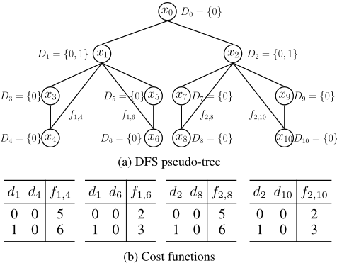
Figure 1 shows the DFS pseudo-tree and cost functions of a DCOP in which the counterexample to termination occurs. The cost functions not specified in Figure 1(b) are defined as the constant functions whose values are 0. In the DCOP, only two agents x1 and x2 have the domain {0, 1}, and the other agents always take the same value, 0.
Trace of the Counterexample
In the trace of this counterexample, agents repeat the transition of their states; in particular, agents x1 and x2 change their variable values infinitely, which results in nontermination and contradicts Property 2 in the original study of ADOPT. Here, the states of some agents at the initial step of the iteration (and the trace itself) are shown in Figure 2.
In the following description, we only focus on the variable values, contexts, lower bounds, and thresholds, which are directly related to this trace, and ignore the rest unless otherwise noted.
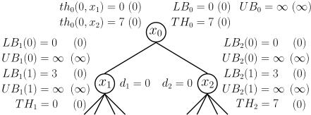
Step 0. As the initial state, we assume that agents x1 and x2 set their values (i.e., d1 and d2) to 0. In the initialization, the thresholds allocated to the children of x0 (i.e., th0(0, x1) and th0(0, x2)) are set to 0; the lower bounds of x1 and x2 (i.e., LB1(0), LB1(1), LB2(0), and LB2(1)) are set to 0; and the thresholds of x1 and x2 (i.e., TH1 and TH2) are set to 0. The states of agents at this point are presented inside the parentheses in Figure 2.
Step 1. Let us begin with the process in the subtree rooted at x1. First, x1 sends VALUE messages to its children and pseudo-children x3, x4, x5, and x6. Afterwards, x4 receives the VALUE message and computes the lower bound using the updated context CX4 ∋ (x1, 0), and thus LB4 = 5. Then x4 reports the lower bound to x3 by sending a COST message. Subsequently, x3 receives the VALUE message from x1 and the COST message from x4 and computes the lower bound as LB3 = 5. Then x3 sends a COST message with CX3 ∋ (x1, 0) and LB3 = 5 to x1. After x1 receives the COST message, x1 updates LB1(0) to 5. Since LB1(0) = 5 > TH1 = 0, x1 changes its value d1 to 1 and sends VALUE messages to its children and pseudo-children.
Step 2. Next, x5 receives the VALUE messages from x1 and sends a COST message to x1, but this COST message does not affect the bounds of x1 because LB5 = 0 and UB5 = ∞, which are the initial bounds. This message is necessary for sending the reinitialized bounds of x5 to x1 in the second or subsequent iteration. Similar to the procedure in Step 1, x1, x3, and x4 receive and send messages, and then x1 updates the lower bound as LB1(1) = 6. Additionally, the threshold of x1 increases as TH1 = LB1 = min{LB1(0), LB1(1)} = 5 because of ThresholdInvariant (for more information on the invariants concerning thresholds, see Appendix A or [Modi et al., 2005]). Since LB1(1) = 6 > TH1 = 5, x1 changes its value d1 back to 0.
Step 3. Subsequently, similar cost calculations and value changes are performed between x1, x5, and x6, and the results are summarized as follows. First, x1 computes the lower bound as LB1(0) = lb1(0, x3) + lb1(0, x5) = 5 + 2 = 7 and then changes its value d1 from 0 to 1. Next, x1 also computes the lower bound as LB1(1) = lb1(1, x3)+lb1(1, x5) = 6 + 3 = 9, and then the value d1 returns to 0. After the cost calculation, x1 sends VALUE messages with the current value d1 = 0 to the lower neighbors and a COST message with LB1 = 7 to x0. Afterwards, x0 receives the COST message and then increases LB0, TH0, and th0(0, x1)
to 7 (the thresholds change due to ThresholdInvariant and ChildThresholdInvariant). As the result of processes from Step 0 to Step 3, the current contexts of the lower neighbors of x1 (i.e., x3, x4, x5, and x6) contain assignment (x1, 1). Note that the lower neighbors of x1 still do not receive the last VALUE messages with d1 = 0 from x1; in particular, x3 and x4 still do not receive the VALUE messages that x1 sent during the processes of x5 and x6 after x3 had sent a COST message to x1 in Step 2.
Step 4. Here, x3 receives the three VALUE messages from x1, in which the values are d1 = 0, d1 = 1, and d1 = 0, in the order of sending. When x3 processes the first VALUE message, the lower bound of x3 is reinitialized as LB3 = LB3(0) = lb3(0, x4) = 0 since context cx3(0, x4) ∋ (x1, 1), received from x4 through the COST message, is incompatible with the updated context CX3 ∋ (x1, 0). After x3 processes the remaining messages, x3 sends two types of COST messages to x1, i.e., the message with LB3 = 0 and CX3 = {(x1, 0)} and the message with LB3 = 0 and CX3 = {(x1, 1)}. Similarly, x5 receives the VALUE message with d1 = 0 from x1 and reinitializes the bounds. Additionally, x5 sends a COST message with LB5 = 0 and CX5 = {(x1, 0)} to x1.
Step 5. Next, x1 receives the COST messages from x3 and x5 and updates the lower bounds as LB1(0) = lb1(0, x3) + lb1(0, x5) = 0, LB1(1) = lb1(1, x3) + lb1(1, x5) = 3. Thus, x1 obtains the lower bound as LB1 = 0 and keeps the value d1 = 0. After x1 sends a COST message with LB1 = 0 to x0, x0 receives it and updates the lower bound as LB0 = LB0(0) = lb0(0, x1) + lb0(0, x2) = 0. Although LB0 decreases, the thresholds for the children are kept as th0(0, x1) = 7 and th0(0, x2) = 0.
Step 6. After the procedures are completed in the subtree rooted at x1, the same process is performed in the subtree rooted at x2. The states of agents after performing the process are presented in Figure 2 (outside the parentheses). In this process, x2 changes its value d2 repeatedly, and eventually the lower bounds of x2 are obtained as LB2(0) = 0 and LB2(1) = 3, and thus LB2 = 0. Here, the thresholds of x0 are crucial. Since x2 once increased LB2 to 7, x0 also increased th0(0, x2) to 7. However, the threshold TH0 has not been changed from 7 because LB0 = lb0(0, x1) + lb0(0, x2) = 0 + 7 = 7. Thus, x0 decreases th0(0, x1) to 0 by AllocationInvariant. Hence, x0 does not satisfy the termination condition since TH0 = 7 < UB0 = ∞ (as x0 received the reinitialized upper bound UB1 = ∞ from x1). Thus, no agent terminates at this point.
Subsequent Steps. Afterwards, the subtrees rooted at x1 and x2 alternately repeat the same process as described from Step 1 to Step 6. This causes x1 and x2 to change their values (i.e., d1 and d2) infinitely; ADOPT never terminates because the root agent x0 never satisfies the termination condition. This result contradicts Property 2.
Cause of the Counterexample
The cause of this counterexample is the nonmonotonicity of lower bounds. In the trace demonstrated above, the lower bounds of x1 and x2 (i.e., LB1 and LB2) increase from 0 to 7
| d0 | d2 | f0,2 |
| 0 | 0 | 100 |
| 0 | 1 | 100 |
| 1 | 0 | 100 |
| 1 (b) | 1 Cost | 0 function |
and then decrease to 0. This transition causes x0 to repeatedly change the thresholds allocated to x1 and x2 (i.e., th0(0, x1) and th0(0, x2)) without altering TH0. Thus, x1 and x2 keep changing their values, and x0 does not satisfy the termination condition.
Occurrence in Variants
Similar counterexamples to termination appear in the variants ADOPT-N and ADOPT+. ADOPT-N is equivalent to the original ADOPT if the given DCOP does not contain nary (n > 2) cost functions. Since the problem consists of only binary functions, ADOPT-N has this flaw. ADOPT+ is a variant of ADOPT that saves its redundant messages. Although the trace above contains redundant messages, a similar trace can be performed without such messages. Therefore, this flaw can appear in ADOPT+.
On the other hand, the counterexample does not occur in IDB-ADOPT. The algorithm repeats the execution of ADOPT, decreasing the initial threshold of the root agent, and eventually, the initial threshold becomes less than the optimal cost by 1. In the DCOP shown in Figure 1, the initial threshold of the root agent at the final execution is 13, and hence the threshold of x1 or x2 must be equal to or greater than 7. Therefore, the agents cannot change their variable values repeatedly, that is, the counterexample does not appear in IDB-ADOPT. Additionally, BnB-ADOPT, BnB-ADOPT+, ADOPT(k), and BD-ADOPT do not have the flaw because the bounds are updated monotonically in these algorithms.
3.2 Counterexample to Optimality Caused by Initialization
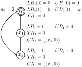
The DFS pseudo-tree and cost function of a DCOP for the second counterexample are shown in Figure 3. The domains of agents x0 and x2 are {0, 1}, and that of agent x1 is {0}. The cost between x0 and x2 is 0 when the two variable values are 1, otherwise, it is 100. Similar to the DCOP for the counterexample to termination, the other cost functions are the constant functions whose values are 0. Thus, the optimal solution of this DCOP is (x0, x1, x2) = (1, 0, 1), whose cost is 0.
Trace of the Counterexample
In this counterexample, a delay of a VALUE message causes termination with a suboptimal solution. The states of agents when x0 terminates (in Step 2) are shown in Figure 4.
Step 0. We assume that all agents set their variable values to 0 in the initialization. At this point, their current contexts are initialized to be empty.
Step 1. First, agents send VALUE messages to their children and pseudo-children. Then x2 receives the VALUE message only from its parent x1, which means that the messages from the pseudo-parent x0 are delayed. Here, x2 updates the current context as CX2 = {(x1, 0)}. From the definition of the local cost δi(d,CX) (see Appendix A), x2 computes the local costs as δ2(0, {(x1, 0)}) = f1,2(0, 0) = 0 and δ2(1, {(x1, 0)}) = f1,2(0, 1) = 0. Thus, the bounds of x2 are obtained as LB2 = UB2 = 0. Then x2 sends a COST message with LB2 = UB2 = 0 to x1.
Step 2. After x1 receives the VALUE message from x0 and the COST message from x2, x1 computes the bounds as LB1 = UB1 = 0. Similarly, x0 updates the bounds as LB0(0) = UB0(0) = 0 through the COST message sent from x1. Since LB0 = TH0 = UB0 = UB0(0) = 0 due to ThresholdInvariant, x0 keeps its value as d0 = 0 and satisfies the termination condition. However, the variable value d0 = 0 is suboptimal. This is a contradiction to Property 3.
Cause of the Counterexample
This counterexample occurs due to the initialization of the current context CXi of agent xi. Since CXi is initialized as an empty set, it may not contain the assignments of some higher neighbors, resulting in an underestimation of the local cost δi(d,CX) and the bounds of xi's ancestors. This fact contradicts Property 1. Moreover, the underestimation results in premature termination.
Occurrence in Variants
This counterexample can occur in ADOPT-N and ADOPT+ since the DCOP contains only binary cost functions and no redundant messages exist in the trace. IDB-ADOPT also encounters this flaw because the initial threshold of the root agent at the final iteration is less than (or essentially equal to) that in ADOPT.
In BnB-ADOPT, BnB-ADOPT+, ADOPT(k), and BDADOPT, the counterexample does not occur since a current context is initialized to contain the assignments of all of the higher neighbors.
3.3 Counterexample to Optimality Caused by TERMINATE Messages
The third counterexample occurs in a DCOP whose DFS pseudo-tree and cost functions are shown in Figure 5. In this DCOP, three agents x0, x2, and x3 have the domain {0, 1}, while the other agents only take values 0. As shown in Figure 5(c), the cost functions f0,3 and f2,3 involved by x3 can be considered as one cost function f0,2 between x0 and x2 since x3 chooses its variable value to minimize the sum of the cost functions, that is, x3 chooses the same value as x0. Note that f0,2 is calculated by x3 and depends on the assignments of x0 and x2 in the current context of x3. Similar to the counterexamples previously shown in this section, the cost functions not specified in Figure 5(b) are the constant functions whose values are 0. The optimal solution of the DCOP is (x0, x1, x2, x3, x4) = (0, 0, 0, 0, 0), whose cost is 1.
Trace of the Counterexample
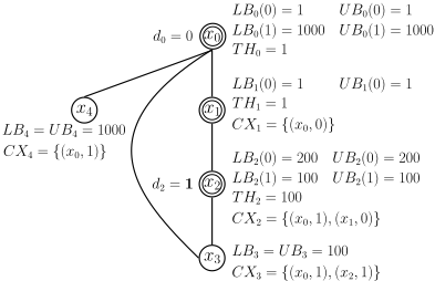
In the DCOP, agent x2 can terminate with a suboptimal value because the termination condition is satisfied despite an incorrect threshold. The states of agents in Step 6, where x2 terminates, are shown in Figure 6.
Step 0. Similar to the other counterexamples, let us assume that all agents set the variable values to 0 as the initial states. First, agents calculate the cost in the case where x0 takes the value 0. We omit this procedure, which is presented in Appendix B. The calculation of the cost results in the following: LB0(0) = UB0(0) = 1; LB0(1) = 0; UB0(1) = ∞; TH0 = 0; TH1 = 1; LB2 = UB2 = 1; TH2 = 1; and d2 = 0. Furthermore, the contexts of the agents except x0 contain assignment (x0, 0). After the calculation, since LB0(0) = 1 > TH0 = 0, x0 changes its value d0 to 1 and sends VALUE messages to x1, x3, and x4.
Step 1. Next, x3 and x4 receive the VALUEmessages from x0. At this moment, x3 updates the context and bounds as CX3 = {(x0, 1), (x2, 0)} and LB3 = UB3 = 200, and x4 also updates them as CX4 = {(x0, 1)} and LB4 = UB4 = 1000. Then they send COST messages to their parents: from x3 to x2 and from x4 to x0. After x0 receives the COST message from x4, x0 changes its value d0 back to 0 since the bounds are obtained as LB0(1) = 1000 and LB0 = TH0 = UB0 = UB0(0) = 1 due to ThresholdInvariant. Therefore, x0 satisfies the termination condition and then terminates. Here, x0 sends VALUE messages with d0 = 0 to its lower neighbors (i.e., x1, x3, and x4) and THRESHOLD and TERMINATE messages to its children (i.e., x1 and x4) in this order, and then x0 executes termination.
Step 2. Afterwards, x1 receives the VALUEmessages from x0, including the message that x0 sent when d0 = 1, in the order of sending. Then x1 changes CX1 from {(x0, 0)} into {(x0, 1)} and returns it to {(x0, 0)}. Since {(x0, 1)} is incompatible with cx1(0, x2) = {(x0, 0)}, x1 reinitializes the bounds as LB1 = 0 and UB1 = ∞. By contrast, TH1 is not changed from 1. Furthermore, x1 receives the THRESHOLD and TERMINATE messages from x0, and then x1 records receiving the TERMINATE message but does not terminate because TH1 = 1 < UB1 = ∞. Subsequently, x1 sends a VALUE message to x2.
| d0 | d3 | f0,3 | d2 | d3 | f2,3 | ||
| 0 | 0 | 1 | 0 0 1 | 0 100 | d0 | d2 f0,2 | |
| 0 1 | 1 0 | 1000 1000 | 0 1 | 10 | 0 | 1 | |
| 1 | 1 | 100 | 0 1 1 | 0 | 0 | 0 1 11 | |
| d0 d4 | f0,4 | 1 1 | 0 200 1 100 | ||||
| 0 | 0 | ||||||
| 0 1 0 | 1000 | ||||||
| (a) DFS pseudo-tree (b) Cost | functions | (c) Cost function induced by f0,3, | |||||
Step 3. Afterwards, x2 receives only the message from x1, not from x3, which means that the messages from x3 are delayed. Then x2 sends a COST message to x1 with CX2 = {(x0, 0), (x1, 0)} and LB2 = UB2 = 1, which are the same states as in Step 0.
Step 4. Next, x2 receives the COST message from x3 with CX3 = {(x0, 1), (x2, 0)} and LB3 = UB3 = 200. Since x2 is not a neighbor of x0, x2 updates CX2 from {(x0, 0), (x1, 0)} to {(x0, 1), (x1, 0)}. Then the bounds of x2 are reinitialized and updated by the bounds in the message: LB2(0) = UB2(0) = 200, LB2(1) = 0, and UB2(1) = ∞. x2 also changes its value d2 to 1 because LB2(0) > TH2 = 1, and sends a VALUE message to x3. After x3 receives only the VALUE message from x2 but not the messages from x1, x3 updates the current context and the bounds as CX3 = {(x0, 1), (x2, 1)} and LB3 = UB3 = 100. Next, x3 sends a COST message to x2 again, and x2 receives it. Then x2 computes the bounds as LB2(1) = UB2(1) = 100 and updates the threshold as TH2 = 100 because of ThresholdInvariant.
Step 5. Here, x1 receives the COST message with CX2 = {(x0, 0), (x1, 0)} and LB2 = UB2 = 1, sent from x2 in Step 3. Since this context is compatible with CX1 = {(x0, 0)}, x1 updates the bounds as LB1 = UB1 = 1. At this moment, the termination condition is satisfied because TH1 = UB1 = 1. Thus, x1 sends two messages to x2: a THRESHOLD message with th1(0, x2) = 1 and CX1 = {(x0, 0)} and a TERMINATE message with CX1 ∪ {(x1, 0)} = {(x0, 0), (x1, 0)}. Then x1 terminates.
Step 6. When x2 receives the THRESHOLDmessage from x1, x2 does not update TH2 since context {(x0, 0)} in the message is incompatible with CX2 = {(x0, 1), (x1, 0)}, and therefore retains its threshold as TH2 = 100. Next, x2 receives the TERMINATE message from x1. Although CX2 is changed to {(x0, 0), (x1, 0)}, the bounds of x2 are not changed since reinitialization is not performed when an agent receives a TERMINATE message. Therefore, x2 terminates with the suboptimal value d2 = 1 because x2 has already satisfied the termination condition with UB2 = UB2(1) = TH2 = 100 and received the TERMINATE message. This result contradicts Property 3.
Cause of the Counterexample
The counterexample presented above is attributed to the following two factors. The first cause is that an agent does not reinitialize its bounds when it receives a TERMINATE message whose context is incompatible with the current context.
However, as shown below, termination with a suboptimal solution can occur even if reinitialization was performed. To demonstrate this fact, let us consider a scenario that the bounds of x2 are reinitialized when x2 receives the TERMINATE message from x1 in Step 6. In this case, the bounds of x2 are obtained as LB2(0) = LB2(1) = 0 and UB2(0) = UB2(1) = ∞; and the threshold of x2 is maintained as TH2 = 100. After x3 receives the VALUE message with the value d0 = 0 from x0, x3 updates the current context as CX3 = {(x0, 0), (x2, 1)} and the bounds as LB3 = UB3 = 11. Then x3 sends a COST message to x2, and x2 receives it. At this point, x2 computes the bounds as LB2(1) = UB2(1) = 11 because context {(x0, 0), (x2, 1)} in the COST message is compatible with CX2 = {(x0, 0), (x1, 0)}. Then x2 updates the threshold as TH2 = 11 due to ThresholdInvariant. Since UB2 = UB2(1) = TH2, x2 does not change its variable value d2 from 1. Therefore, x2 satisfies the termination condition and terminates with the suboptimal value d2 = 1.
The second cause of the counterexample is an incorrect threshold at termination. Even if the threshold of an agent differs from that in the THRESHOLD message sent just before a TERMINATE message, the termination condition of the agent can be satisfied. Therefore, the agent can terminate with a suboptimal value.
Occurrence in Variants
In ADOPT-N and IDB-ADOPT, this counterexample occurs for the same reasons as the flaws previously shown. Moreover, BnB-ADOPT, BnB-ADOPT+, ADOPT(k), and BDADOPT all have similar flaws. The causes of them are that agents do not send their current contexts in VALUE messages, which include thresholds, or TERMINATE messages. Thus, they can terminate with incorrect contexts.
The incorrectness of contexts means that the statements of the proofs in the studies of ADOPT(k) and BD-ADOPT are not appropriate. They imply that agents obtain the optimal costs for each of the current contexts, which may be incorrect at termination. The study of BnB-ADOPT also presents an inappropriate statement. It implies that only the root agent obtains the optimal cost at termination, however, the other agents can terminate with incorrect contexts, resulting in a suboptimal solution.
By contrast, ADOPT+ does not have this flaw because it is obtained by fixing the causes of the flaw in ADOPT. Specifically, in ADOPT+, a VALUE message contains the current context and threshold of the agent, and furthermore, a time stamp for a variable value is introduced. These modifications guarantee the correct context and threshold at termination, and agents can reinitialize the bounds if the current context is changed.
4 Amendment to ADOPT
In this section, we propose an amended version of ADOPT to avoid the flaws. The amendment consists of three parts, each of which corresponds to one of the causes described in Section 3. The pseudocode of our version of ADOPT is presented in Appendix C.
First, we modify the update rules for the lower and upper bounds lbi(d, xc) and ubi(d, xc) for a child so as to change monotonically. In the amended version, when agent xi receives a COST message from child xc with bounds LBc and UBc and context CXc ∋ (xi, d), xi updates the lower and upper bounds for d and xc by the following:
The other calculations of the lower and upper bounds (i.e., LBi(d),UBi(d),LBi, and UBi) are not changed from the original definitions.
Second, we modify the initialization of a current context so as to store the assignments of all higher neighbors. Agent xi initializes the current context as follows:
where V alInit(xp) ∈ Dp is the initial value for xp and SCP(xi) is a set of the ancestors of xi that are parents or pseudo-parents of agents (including xi) in the subtree rooted at xi. Note that for xi to avoid flaws, it is sufficient to initialize the current context with the assignments of the parent and pseudo-parents of xi. However, our amended version uses the assignments of all agents in SCP(xi) since the current context CXi eventually stores their assignments. The two aforementioned amendments have been introduced in BnBADOPT, BnB-ADOPT+, ADOPT(k), and BD-ADOPT.
Finally, we modify TERMINATE messages and their receiving procedure. The amended procedure when agent xi receives a TERMINATE message from the parent xp is as follows: if the context cxi(d, xc) for value d and child xc is incompatible with the current context CXi updated by the TERMINATE message, xi reinitializes the lower and upper bounds lbi(d, xc) and ubi(d, xc), threshold thi(d, xc), and context cxi(d, xc). Additionally, we introduce the threshold thi(di, xc) for the current value di and child xc into the TERMINATE message sent to xc. The amendment to TERMINATE messages guarantees the threshold of an agent after receiving a TERMINATE message to be correct, which is proven by a theorem in the next section. Therefore, the termination condition is satisfied with the correct threshold and optimal value.
5 Proof of Termination and Optimality
Our amended algorithm guarantees termination and optimality, which are stated as Theorems 1 and 2 below, and the full proofs and lemmata are shown in Appendix D. The arguments of the proofs are based on the study of BnB-ADOPT. However, the statements of the theorems are modified to derive our aimed properties.
For the theorem of optimality, we define the correctness of the current context of an agent.
Definition 1. The current context CXi of agent xi is correct iff CXi contains the assignments of all agents in SCP(xi), and the values of all agents in CXi are equal to the values of the agents.
The theorems for the amended version of ADOPT are as follows:
Theorem 1. The amended version of ADOPT terminates after a finite amount of time.
Theorem 2. For any agent xi ∈ X when the amended version of ADOPT terminates, the current context CXi is correct, and THi = γi(di, CXi) = γi(CXi).
6 Conclusion
We presented flaws in ADOPT and its variants with respect to termination and optimality, which have been believed to be correct. The flaws are classified into three types, one of which is related to termination, while the other two of which are related to optimality. The causes of the flaws are the update rules for the bounds, the initialization of a current context, and TERMINATE messages and their receiving procedure. Additionally, we proposed an amended version of ADOPT that avoids these flaws, whose amendment corresponds to the causes of the flaws. Furthermore, we proved termination and optimality in the amended version of ADOPT. For future work, we plan to verify the properties of ADOPT-ing, which was not analyzed in this work.
@inproceedings{ijcai2023p222,
  title     = {Flaws of Termination and Optimality in ADOPT-based Algorithms},
  author    = {Noshiro, Koji and Hasebe, Koji},
  booktitle = {Proceedings of the Thirty-Second International Joint Conference on
               Artificial Intelligence, {IJCAI-23}},
  publisher = {International Joint Conferences on Artificial Intelligence Organization},
  editor    = {Edith Elkind},
  pages     = {1996--2003},
  year      = {2023},
  month     = {8},
  note      = {Main Track},
  doi       = {10.24963/ijcai.2023/222},
  url       = {https://doi.org/10.24963/ijcai.2023/222},
}
TY - CPAPER TI - Flaws of Termination and Optimality in ADOPT-based Algorithms AU - Noshiro, Koji AU - Hasebe, Koji T2 - Proceedings of the Thirty-Second International Joint Conference on Artificial Intelligence, IJCAI-23 PB - International Joint Conferences on Artificial Intelligence Organization PY - 2023 SP - 1996 EP - 2003 DO - 10.24963/ijcai.2023/222 UR - https://doi.org/10.24963/ijcai.2023/222 ER -Copied
Machine-readable versions of this paper, for tools and AI agents:





