
SMARTformer: Semi-Autoregressive Transformer with Efficient Integrated Window Attention for Long Time Series Forecasting
Proceedings of the Thirty-Second International Joint Conference on Artificial Intelligence. Main Track. Pages 2169-2177.
https://doi.org/10.24963/ijcai.2023/241
Keywords
- Data Mining: DM: Mining spatial and/or temporal data
- Data Mining: DM: Applications
- Machine Learning: ML: Regression
- Machine Learning: ML: Time series and data streams
Abstract
The success of Transformers in long time series forecasting (LTSF) can be attributed to their attention mechanisms and non-autoregressive (NAR) decoder structures, which capture long-range de- pendencies. However, time series data also contain abundant local temporal dependencies, which are often overlooked in the literature and significantly hinder forecasting performance. To address this issue, we introduce SMARTformer, which stands for SeMi-AutoRegressive Transformer. SMARTformer utilizes the Integrated Window Attention (IWA) and Semi-AutoRegressive (SAR) Decoder to capture global and local dependencies from both encoder and decoder perspectives. IWA conducts local self-attention in multi-scale windows and global attention across windows with linear com- plexity to achieve complementary clues in local and enlarged receptive fields. SAR generates subsequences iteratively, similar to autoregressive (AR) decoding, but refines the entire sequence in a NAR manner. This way, SAR benefits from both the global horizon of NAR and the local detail capturing of AR. We also introduce the Time-Independent Embedding (TIE), which better captures local dependencies by avoiding entanglements of various periods that can occur when directly adding po- sitional embedding to value embedding. Our ex- tensive experiments on five benchmark datasets demonstrate the effectiveness of SMARTformer against state-of-the-art models, achieving an improvement of 10.2% and 18.4% in multivariate and univariate long-term forecasting, respectively.
- [Ba et al., 2016] Jimmy Lei Ba, Jamie Ryan Kiros, and Ge- offrey E Hinton. Layer normalization. arXiv preprint arXiv:1607.06450, 2016.
- [Bai et al., 2020] Lei Bai, Lina Yao, Can Li, Xianzhi Wang, and Can Wang. Adaptive graph convolutional recurrent network for traffic forecasting. Advances in neural infor- mation processing systems, 33:17804-17815, 2020.
- [Chen et al., 2022] Weiqi Chen, Wenwei Wang, Bingqing Peng, Qingsong Wen, Tian Zhou, and Liang Sun. Learning to rotate: Quaternion transformer for complicated period- ical time series forecasting. In Proceedings of the 28th ACM SIGKDD Conference on Knowledge Discovery and Data Mining, pages 146-156, 2022.
- [Cirstea et al., 2022] Razvan-Gabriel Cirstea, Chenjuan Guo, Bin Yang, Tung Kieu, Xuanyi Dong, and Shirui Pan. Triformer: Triangular, variable-specific attentions for long sequence multivariate time series forecasting. In Luc De Raedt, editor, Proceedings of the Thirty-First International Joint Conference on Artificial Intelligence, IJCAI 2022, Vienna, Austria, 23-29 July 2022, pages 1994-2001. ijcai.org, 2022. IJCAI
- [Deng et al., 2021] Jinliang Deng, Xiusi Chen, Renhe Jiang, Xuan Song, and Ivor W Tsang. St-norm: Spatial and tem- poral normalization for multi-variate time series forecast- ing. In Proceedings of the 27th ACM SIGKDD conference on knowledge discovery & data mining, pages 269-278, 2021.
- [Gu et al., 2017] Jiatao Gu, James Bradbury, Caiming Xiong, Victor OK Li, and Richard Socher. Non- autoregressive neural machine translation. arXiv preprint arXiv:1711.02281, 2017.
- [Gu et al., 2022] Albert Gu, Karan Goel, and Christopher Ré. Efficiently modeling long sequences with struc- tured state spaces. In The Tenth International Conference on Learning Representations, ICLR 2022, Virtual Event, April 25-29, 2022. OpenReview.net, 2022.
- [Hochreiter and Schmidhuber, 1997] Sepp Hochreiter and Jürgen Schmidhuber. Long short-term memory. Neural computation, 9(8):1735-1780, 1997.
- [Kim et al., 2022] Taesung Kim, Jinhee Kim, Yunwon Tae, Cheonbok Park, Jangho Choi, and Jaegul Choo. Re- versible instance normalization for accurate time-series forecasting against distribution shift. In ICLR, 2022.
- [Kingma and Ba, 2015] Diederik P. Kingma and Jimmy Ba. Adam: A method for stochastic optimization. In Yoshua Bengio and Yann LeCun, editors, 3rd International Con- ference on Learning Representations, ICLR 2015, San Diego, CA, USA, May 7-9, 2015, Conference Track Pro- ceedings, 2015.
- [Kitaev et al., 2020] Nikita Kitaev, Lukasz Kaiser, and Anselm Levskaya. Reformer: The efficient transformer. In 8th International Conference on Learning Represen- tations, ICLR 2020, Addis Ababa, Ethiopia, April 26-30, 2020. OpenReview.net, 2020.
- [Lai et al., 2018] Guokun Lai, Wei-Cheng Chang, Yiming Yang, and Hanxiao Liu. Modeling long-and short-term temporal patterns with deep neural networks. In The 41st international ACM SIGIR conference on research & devel- opment in information retrieval, pages 95-104, 2018.
- [Lewis et al., 2019] Mike Lewis, Yinhan Liu, Naman Goyal, Marjan Ghazvininejad, Abdelrahman Mohamed, Omer Levy, Ves Stoyanov, and Luke Zettlemoyer. Bart: De- noising sequence-to-sequence pre-training for natural lan- guage generation, translation, and comprehension. arXiv preprint arXiv:1910.13461, 2019.
- [Li et al., 2018] Yaguang Li, Rose Yu, Cyrus Shahabi, and Yan Liu. Diffusion convolutional recurrent neural net- work: Data-driven traffic forecasting. In 6th Interna- tional Conference on Learning Representations, ICLR 2018, Vancouver, BC, Canada, April 30 -May 3, 2018, Conference Track Proceedings. OpenReview.net, 2018.
- [Li et al., 2019] Shiyang Li, Xiaoyong Jin, Yao Xuan, Xiyou Zhou, Wenhu Chen, Yu-Xiang Wang, and Xifeng Yan. En- hancing the locality and breaking the memory bottleneck of transformer on time series forecasting. Advances in neu- ral information processing systems, 32, 2019.
- [Li et al., 2021] Fuxian Li, Jie Feng, Huan Yan, Guangyin Jin, Fan Yang, Funing Sun, Depeng Jin, and Yong Li. Dynamic graph convolutional recurrent network for traffic prediction: Benchmark and solution. ACM Transactions on Knowledge Discovery from Data (TKDD), 2021.
- [Li et al., 2023a] Zhe Li, Zhongwen Rao, Lujia Pan, Pengyun Wang, and Zenglin Xu. Ti-mae: Self-supervised masked time series autoencoders. CoRR, abs/2301.08871, 2023.
- [Li et al., 2023b] Zhe Li, Zhongwen Rao, Lujia Pan, and Zenglin Xu. Mts-mixers: Multivariate time series forecast- ing via factorized temporal and channel mixing. CoRR, abs/2302.04501, 2023.
- [Liu et al., 2018] Hao Liu, Lirong He, Haoli Bai, Bo Dai, Kun Bai, and Zenglin Xu. Structured inference for re- current hidden semi-markov model. In Proceedings of the Twenty-Seventh International Joint Conference on Ar- tificial Intelligence, IJCAI 2018, July 13-19, 2018, Stock- holm, Sweden, pages 2447-2453, 2018. IJCAI
- [Liu et al., 2021] Shizhan Liu, Hang Yu, Cong Liao, Jian- guo Li, Weiyao Lin, Alex X Liu, and Schahram Dust- dar. Pyraformer: Low-complexity pyramidal attention for long-range time series modeling and forecasting. In Inter- national Conference on Learning Representations, 2021.
- [Liu et al., 2022] Yong Liu, Haixu Wu, Jianmin Wang, and Mingsheng Long. Non-stationary transformers: Rethink- ing the stationarity in time series forecasting. arXiv preprint arXiv:2205.14415, 2022.
- [Paszke et al., 2019] Adam Paszke, Sam Gross, Francisco Massa, Adam Lerer, James Bradbury, Gregory Chanan, Trevor Killeen, Zeming Lin, Natalia Gimelshein, Luca Antiga, et al. Pytorch: An imperative style, high- performance deep learning library. Advances in neural in- formation processing systems, 32, 2019.
- [Qin et al., 2017] Yao Qin, Dongjin Song, Haifeng Chen, Wei Cheng, Guofei Jiang, and Garrison W. Cottrell. A dual-stage attention-based recurrent neural network for time series prediction. In Carles Sierra, editor, Proceed- ings of the Twenty-Sixth International Joint Conference on Artificial Intelligence, IJCAI 2017, Melbourne, Australia, August 19-25, 2017, pages 2627-2633. ijcai.org, 2017. IJCAI
- [Salinas et al., 2020] David Salinas, Valentin Flunkert, Jan Gasthaus, and Tim Januschowski. Deepar: Probabilistic forecasting with autoregressive recurrent networks. Inter- national Journal of Forecasting, 36(3):1181-1191, 2020.
- [Shabani et al., 2022] Amin Shabani, Amir Abdi, Lili Meng, and Tristan Sylvain. Scaleformer: Iterative multi-scale refining transformers for time series forecasting. CoRR, abs/2206.04038, 2022.
- [Sun and Boning, 2022] Fan-Keng Sun and Duane S Bon- ing. Fredo: Frequency domain-based long-term time se- ries forecasting. arXiv preprint arXiv:2205.12301, 2022.
- [Sutskever et al., 2014] Ilya Sutskever, Oriol Vinyals, and Quoc V. Le. Sequence to sequence learning with neural networks. In Zoubin Ghahramani, Max Welling, Corinna Cortes, Neil D. Lawrence, and Kilian Q. Weinberger, edi- tors, Advances in Neural Information Processing Systems 27: Annual Conference on Neural Information Processing Systems 2014, December 8-13 2014, Montreal, Quebec, Canada, pages 3104-3112, 2014.
- [Vaswani et al., 2017] Ashish Vaswani, Noam Shazeer, Niki Parmar, Jakob Uszkoreit, Llion Jones, Aidan N Gomez, Łukasz Kaiser, and Illia Polosukhin. Attention is all you need. Advances in neural information processing systems, 30, 2017.
- [Wu et al., 2019] Zonghan Wu, Shirui Pan, Guodong Long, Jing Jiang, and Chengqi Zhang. Graph wavenet for deep spatial-temporal graph modeling. In Sarit Kraus, edi- tor, Proceedings of the Twenty-Eighth International Joint Conference on Artificial Intelligence, IJCAI 2019, Macao, China, August 10-16, 2019, pages 1907-1913. ijcai.org, 2019. IJCAI
- [Wu et al., 2021] Haixu Wu, Jiehui Xu, Jianmin Wang, and Mingsheng Long. Autoformer: Decomposition transform- ers with auto-correlation for long-term series forecast- ing. Advances in Neural Information Processing Systems, 34:22419-22430, 2021.
- [Yang et al., 2019] Zhilin Yang, Zihang Dai, Yiming Yang, Jaime Carbonell, Russ R Salakhutdinov, and Quoc V Le. Xlnet: Generalized autoregressive pretraining for lan- guage understanding. Advances in neural information pro- cessing systems, 32, 2019.
- [Zeng et al., 2022] Ailing Zeng, Muxi Chen, Lei Zhang, and Qiang Xu. Are transformers effective for time series fore- casting? CoRR, abs/2205.13504, 2022.
- [Zhou et al., 2021] Haoyi Zhou, Shanghang Zhang, Jieqi Peng, Shuai Zhang, Jianxin Li, Hui Xiong, and Wancai Zhang. Informer: Beyond efficient transformer for long sequence time-series forecasting. In Proceedings of the AAAI Conference on Artificial Intelligence, volume 35, pages 11106-11115, 2021.
- [Zhou et al., 2022a] Tian Zhou, Ziqing Ma, Qingsong Wen, Xue Wang, Liang Sun, and Rong Jin. Fedformer: Fre- quency enhanced decomposed transformer for long-term series forecasting. In Kamalika Chaudhuri, Stefanie Jegelka, Le Song, Csaba Szepesvári, Gang Niu, and Sivan Sabato, editors, International Conference on Machine Learning, ICML 2022, 17-23 July 2022, Baltimore, Mary- land, USA, volume 162 of Proceedings of Machine Learn- ing Research, pages 27268-27286. PMLR, 2022.
- [Zhou et al., 2022b] Tian Zhou, Ziqing Ma, Qingsong Wen, Xue Wang, Liang Sun, and Rong Jin. Fedformer: Fre- quency enhanced decomposed transformer for long-term series forecasting. In Kamalika Chaudhuri, Stefanie Jegelka, Le Song, Csaba Szepesvári, Gang Niu, and Sivan Sabato, editors, International Conference on Machine Learning, ICML 2022, 17-23 July 2022, Baltimore, Mary- land, USA, volume 162 of Proceedings of Machine Learn- ing Research, pages 27268-27286. PMLR, 2022.
References were extracted automatically from the PDF and may contain errors.
Full text extracted automatically from the PDF; figures, tables and equations may differ. The PDF is the version of record.
1 Introduction
Multivariate Time Series Forecasting, as an interdisciplinary research prevalent in scientific and engineering problems, has witnessed great advances in recent years, with a notable trend of predicting accurate series from short term [Li et al., 2018; Liu et al., 2018; Salinas et al., 2020; Bai et al., 2020; Deng et al., 2021] to long term [Zhou et al., 2021; Li et al., 2023a; Li et al., 2023b]. Recently, Transformer-based models [Vaswani et al., 2017] have demonstrated great potentials on long time series forecasting (LTSF) for capturing longrange correlations.
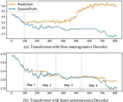
Despite these potentials, existing transformer-based models do not adequately consider the characteristics of time series data and are still suffering from ineffectiveness and inefficiency in capturing those local dependencies among complicated temporal patterns, impairing the ability to accurately model long time series. For instance, as shown in Figure 1a, when predicting a long time sequence with a size of 720 timesteps for the real-world Exchange-rate dataset [Lai et al., 2018], the non-stationary transformer [Liu et al., 2022] with a typical non-autoregressive decoder, leads to performance collapse in a single prediction step.
Moreover, positional embedding is also directly related to local dependencies. Due to the different scales in time series, directly adding positional embedding to the value embedding, as previous works [Zhou et al., 2022a; Wu et al., 2021], can result in entanglements of various periods, thus leading to confusion for future prediction. Therefore, we develop TIE to better capture the local dependencies.
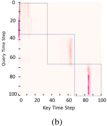
We further investigate the vanilla attention mechanism's limitations by examining the attention maps among different timesteps computed on the Exchange rate dataset (Figure 2b). The attention map is highly sparse, which aligns with recent research [Zhou et al., 2021]. They found that the attention feature map follows a long-tail distribution, where a few dot-product pairs contribute to attentions while most can be ignored. This limited attention mechanism hinders transformer models from learning better temporal correlations among timesteps, leading to significant computation costs that restrict the practical deployment of such models in real-world applications.
In summary, by investigating the architectures of Transformers for time series interaction, there are several major bottlenecks, i.e., the input embeddings that can incorporate more decoupled prior information, the attention mechanism that can efficiently and effectively model the interaction among different temporal patterns, and the decoder that can stably forecast with consistent long-range dependencies.
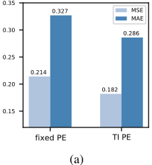
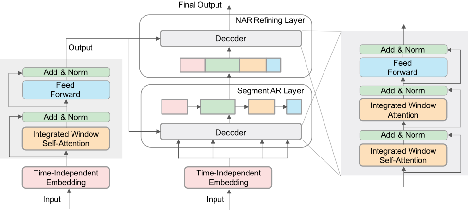
We propose the SMARTformer, which stands for SeMiAutoRegressive Transformer with Efficient Integrated Window Attention, to address issues in general LTSF tasks. The SMARTformer architecture is illustrated in Figure 3. To better decouple positional embedding from value embedding, we design a simple yet effective Time-Independent Embedding (TIE) method, which avoids entanglements of various periods and enhances the inductive bias of significant periodic variations. This improvement is shown on the Electricity Dataset in Figure 2a. To capture abundant latent correlations, we design the Integrated Window Attention (IWA), which separates an attention layer into two branches. One branch conducts local self-attention in non-overlapping multi-scale windows, while the other conducts global attention across windows. These designs achieve valuable temporal patterns (as shown in Table 7) and break the bottleneck of computational efficiency (as demonstrated in Figure 5). Furthermore, to enhance the decoder's power for outputting consistent longrange dependencies, we design a semi-autoregressive (SAR) decoder. The promising performance of SAR is demonstrated in Figure 1b, which enables the non-stationary Transformer to better fit the ground truth sequence. Extensive experiments on five public and commonly used multivariate time series datasets from different domains demonstrate the outstanding performance of the proposed SMARTformer.
2 RelatedWork
We review transformer models for LTSF according to the attention mechanism and decoder design.
Efficient Attentions in LTSF. To tackle LTSF tasks, designing effective self-attention mechanisms is crucial. According to attentions, Transformer variants can be roughly categorized into two types. The first type is Temporal Sparse Attention, which sparsifies attention with predefined patterns [Li et al., 2019; Kitaev et al., 2020; Liu et al., 2021; Cirstea et al., 2022]. Through reducing complexity, they are trapped by prefined structures, failing to accurately capture the correlations. The second type is Frequency Domain Attention, which fuses decomposition blocks with Fast Fourier Transform or other frequency analysis method to discover series-wise connections [Wu et al., 2021; Zhou et al., 2022a; Chen et al., 2022]. However, converting data to frequency domain may inevitably lose fine temporal variations, thus leading to sub-optimal solutions. Based on the data distribution of the attention matrices (as illustrated in Figure 2a), the proposed Integrated Window Attention is designed to model local and global interaction at the same time, which is significantly different from existing methods.
Non-Autoregressive Decoding. Autoregressive (AR) decoding is widely used in NLP seq2seq models [Sutskever et al., 2014] and Transformer-based pretraining models [Lewis et al., 2019; Yang et al., 2019]. Meanwhile, AR decoding dominates in short time series forecasting, [Qin et al., 2017; Salinas et al., 2020; Lai et al., 2018; Li et al., 2019]. However, for LTSF, AR decoding achieves unsatisfactory performance due to error accumulation, as mathematically proven in [Sun and Boning, 2022]. Thus, Informer initially adopted Non-autoregressive (NAR) decoding [Gu et al., 2017] to avoid error accumulation and improve efficiency, which was also used in subsequent works (Autoformer [Wu et al., 2021], FEDformer [Zhou et al., 2022b], and Scaleformer [Shabani et al., 2022]). Although these methods achieved encouraging results by injecting multi-scale or decomposition prior, they still neglected the disadvantages of NAR decoding itself. Our SAR decoder acts orthogonally to their contributions and can be easily adapted to them and other time series transformers to consistently enhance their performance.
3 Method
Given a D-variates time series W = [w1,w2, . . . ,wT ] ∈ RT×D with T timesteps, the LTSF problem aims to predict ˜W = [wT+1,wT+2, . . . ,wT+L] ∈ RL×D with L future timestep values. To tackle the LTSF tasks, we design the architecture of the proposed SMARTformer, as shown in Figure 3. In the following, we introduce the major components, i.e., the Time-Independent Embedding, the Integrated Window Attention, and the hierarchical Semi-autoregressive Decoder.
3.1 Time-Independent Embedding
In transformer-based time series forecasting, data embedding significantly impacts performance because attentions are insensitive to data order. To enhance the awareness of temporal variations, local positional and temporal information is often added [Zeng et al., 2022]. Previous studies use fixed positional encoding or date-specific embedding to maintain ordering information. However, time series data often contain waveforms with different periods. Adding positional encoding composed of periodic waveforms may destroy original values by causing phase cancellation. We propose that positional encoding should be decoupled from values in time series embedding to reduce the distortion of original data.
To this end, we design a Time-Independent (TI) embedding method. Raw historical data are used as the encoder input W1:T = {wi,d | 1 ≤ i ≤ T, 1 ≤ d ≤ D}, where wi,d denotes the i-th timestep in dimension d. For each timestep, we embed them through two parts: theValue Embeddingwith a simple 1-D convolutional layer to embed each timestep of raw data to a Cv dimension vector, and the Time-Independent Positional Embedding denoted by Fi, calculated as the concatanation of three types of temporal features, i.e.,
Here E(m/h) ,E(wk) ,E(mth) denote three learnable projection matrices for positional embeddings of minute/hour, weekday and month, respectively. Fi ∈ R Cp denotes the vector after positional embedding. Thus, the positional information is shared among timesteps of the same order on a daily/weekly/monthly basis to enhance the understanding of global temporal changes.
For each token wi, we concatenate and normalize these two embeddings (following [Ba et al., 2016]) as
where Conv (wi) ∈ RCv denotes the latent variable after Value Embedding and Ei ∈ R C (C = Cv + Cp) denotes the input embedding. In this way, we leverage the positional information without destroying data semantics, acquiring global awareness of ultra-long temporal changes.
3.2 IntegratedWindowAttention
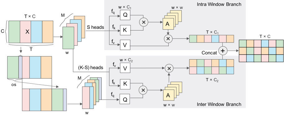
First, the input feature X ∈ R T×C is linearly projected to K heads, and our proposed attention splits them into two groups - one with S heads (for Intra-window attention) and the other with K-S heads (for Inter-window attention).
Intra-window Attention. For attention in windows, X is evenly partitioned into non-overlapping windows of equal length w along the time dimension. Here, we assume w is divisible by the whole length T . w can be adjusted to balance the learning capacity and computation complexity. Therefore, intra-window attention can be defined as
where Xi ∈ R TM ×C and M = T/w (i = 1, 2, . . . ,M). W Q k ∈ R C×dk , W K k ∈ R C×dk , and W V k ∈ R C×dk represent the projection matrices of queries, keys, and values for the k-th head respectively where dk is set as C/K. Besides, the window length w is an important parameter because it achieves strong modeling capability while limiting the computation cost, where we adjust by applying small lengths for shallow layers and larger lengths for deep layers respectively to capture multi-scale characteristics.
Inter-window Attention. For remaining K -S heads, we perform Inter-Attention, where we shift the original sequence X into Xs with os timesteps, and split it through the same window size w as the former branch to acquire ˆX as
The shifted sequence ˆX is projected as Queries and X is projected as Keys and Values. Then, we acquire the k-th head attention scores Y i k for the i-th window as
where e · w < os < (e+1) · w, 0 < e < M. os is an offset to establish powerful connections across different windows and enhance interactions among tokens at the edge of windows. Then, we integrate two branches to acquire the final output as
By doing so, the computation complexity of the Integrated Window Attention in two branches is both O(w × L) = O(L), scaling linearly with the input length L, reducing greatly to a lower complexity than the standard MSA and ensuring high throughput on GPUs. Moreover, another benefit of head-splitting is that the learnable parameters Q, K, and V are decomposed into two smaller matrices, which helps to reduce model parameters. And we apply different w window sizes for different layers, small w for early stages and larger w for later. Adjusting the length of w provides the flexibility to enlarge the attention area of each token. Thus, we reconcile the global and local self-attention in a single layer to acquire ample variations in an efficient and effective way.
3.3 Semi-Autoregressive Decoder
We describe our hierarchical SAR decoder to handle robust long sequence prediction, as shown in Figure 3. It stacks the Segment AR layer and the NAR refining layer. These layers share the identical structure of a typical Transformer decoder, except for using the IWA instead.
Segment AR Layer. Despite focusing on modeling a long sequence, local contexts also play a crucial role in knowledge propagation. Therefore, in the lower section of our network, we adopt a Segment AR Decoder Layer, which predicts each subsequence iteratively by applying the same decoder layer. For a long sequence with a length of L to predict in the M-th decoder layer, it generates non-overlapping segments through k steps with a length lk. And the output of the M-th decoder layer ZM de ∈ R L×C is acquired by concatenating all the kstep representations along the time dimension as
where ˆ Y M de(j) denotes the j-th step output.
In the j-th step, we assume Lj for the predicted length. A local representation HM (j) ∈ R Lj×C takes as the input, which comes from the predictions of previous steps and positional information of current step to capture local fine variations. ¯ Y M de(j-1) ∈ R Lj×C denotes a slice from the previous prediction ˆ Y M de(j-1) ∈ R Lj-1×C which we pad or slice to a proper length when j = 1 or lj-1 ̸= lj to align them in the time dimension. The positional embeddings F(j) ∈ R Lj×Cp utilize TIE to enhance the awareness of complicated periodic variations. We concatenate them along the channel dimension and learn through an MLP as
| Method | SMARTformer | Stationary | DLinear | FEDformer | Autoformer | Informer | LogTrans | LSSL | LSTM | ||||||||||
|---|---|---|---|---|---|---|---|---|---|---|---|---|---|---|---|---|---|---|---|
| Metric | MSE | MAE | MSE | MAE | MSE | MAE | MSE | MAE | MSE | MAE | MSE | MAE | MSE | MAE | MSE | MAE | MSE | MAE | |
| Weather | 96 192 336 720 | 0.171 0.224 0.283 0.361 | 0.224 0.268 0.313 0.358 | 0.190 0.241 0.309 0.406 | 0.237 0.281 0.328 0.394 | 0.196 0.237 0.283 0.375 | 0.255 0.296 0.335 0.381 | 0.217 0.276 0.339 0.403 | 0.296 0.336 0.380 0.428 | 0.266 0.307 0.359 | 0.336 0.367 0.395 | 0.300 0.598 0.578 | 0.384 0.544 | 0.689 0.658 | 0.596 0.589 | 0.174 0.238 0.287 | 0.252 0.313 0.355 0.415 | 0.369 0.416 0.455 0.535 | 0.406 0.435 |
| Traffic | 96 192 336 720 | 0.638 0.163 0.171 0.191 0.203 0.109 | 0.233 0.314 | 0.111 0.239 | 0.237 0.345 | 0.088 0.176 | 0.301 0.333 0.218 | 0.195 0.212 0.246 | 0.355 0.276 | 0.660 0.197 | 0.408 0.317 0.361 | 0.864 | 0.472 | 0.684 0.734 0.717 0.258 | 0.396 0.812 0.851 | 0.317 0.338 0.395 0.776 | 0.489 0.392 0.390 0.403 0.417 | 0.454 0.520 0.453 | |
| 96 | 0.583 0.592 0.608 | 0.421 | 0.476 | 0.315 | 0.193 | 0.297 0.308 0.313 | 0.254 | 0.428 | 1.059 0.777 | 0.523 0.741 | 0.797 0.869 | 0.357 0.368 1.081 | 0.300 0.297 | 0.474 0.698 | 2.136 | ||||
| 192 | 0.317 0.322 0.333 0.346 0.269 0.277 | 0.612 0.613 0.618 0.653 | 0.338 0.340 0.328 0.355 | 0.650 0.598 0.609 0.645 | 0.396 0.370 0.373 0.394 0.282 | 0.587 0.604 0.621 | 0.366 0.373 0.383 | 0.419 0.613 | 0.388 | 0.719 | 0.391 | 0.652 0.675 | 0.384 0.798 0.849 | 0.436 0.481 0.476 | 0.843 0.847 0.853 | 0.453 0.455 0.805 | |||
| Electricity | 336 | 0.177 0.205 | 0.284 0.304 | 0.197 0.196 | 0.285 | 0.641 | 0.382 | 0.616 0.622 | 0.382 0.337 | 0.696 | 0.379 0.420 | 0.685 | 0.384 0.390 0.408 | 0.828 0.854 | 1.500 0.375 | 0.437 0.473 | |||
| 720 | 0.292 0.306 | 0.221 0.244 | 0.324 0.341 | 0.209 0.245 | 0.139 | 0.201 0.222 0.231 | 0.334 0.338 | 0.274 0.298 0.307 0.373 | 0.368 0.389 0.399 0.439 | 0.266 0.280 0.283 | 0.380 0.376 | 0.442 0.439 0.980 | 0.473 0.814 | ||||||
| Exchange | 96 192 | 0.186 | 0.195 | 0.308 | 0.323 | 0.847 | 0.752 | 0.968 | 1.029 | 1.453 1.846 | 1.049 1.179 | ||||||||
| 336 720 | 0.348 | 0.421 0.649 | 1.082 | 0.804 | 0.320 0.839 | 0.427 0.695 | 0.426 | 0.464 | 0.222 | 0.334 0.524 | 1.204 1.672 | 0.895 1.036 | 1.040 1.659 | 2.283 | 0.797 | 1.231 | |||
| 24 | 0.789 | 2.494 | 1.065 | 1.090 | 0.800 | 0.509 | 2.478 | 1.310 | 1.941 | 1.127 | 4.381 | 1.222 | 2.984 | ||||||
| 2.284 | 0.933 | 2.398 | 1.040 | 3.228 | 1.447 | 0.941 | 1.427 | ||||||||||||
| 36 | 1.770 | 1.260 | 3.483 | 1.677 | 5.914 | 1.734 | |||||||||||||
| 5.764 | 1.444 | 1.425 | |||||||||||||||||
| 1.877 | 0.883 | 1.287 | 4.480 | ||||||||||||||||
| 0.845 | 2.646 | 1.088 | 2.679 | 1.080 | 3.103 | 1.148 | 4.755 | 1.467 | 4.799 | 1.467 | 4.442 | 1.416 | 6.631 | 1.845 | |||||
| ILI | |||||||||||||||||||
| 48 | 0.897 | 0.900 | 2.614 | 1.086 | 2.622 | 1.078 | 6.736 | ||||||||||||
| 1.897 | 2.010 | 2.669 | 4.800 | 1.468 | 4.559 | 1.443 | 1.857 | ||||||||||||
| 1.877 | 1.085 | 4.763 | 1.469 | ||||||||||||||||
| 60 | 0.891 | 2.178 | 0.963 | 2.804 | 1.146 | 2.857 | 1.157 | 2.770 | 1.125 | 5.264 | 1.564 | 5.278 | 1.560 | 4.651 | 1.474 | 6.870 | 1.879 | ||
| Method | SMARTformer | Stationary | DLinear | FEDformer | Autoformer | Informer | LogTrans | LSSL | LSTM | ||||||||||
|---|---|---|---|---|---|---|---|---|---|---|---|---|---|---|---|---|---|---|---|
| Metric | MSE | MAE | MSE | MAE | MSE | MAE | MSE | MAE | MSE | MAE | MSE | MAE | MSE | MAE | MSE | MAE | MSE | MAE | |
| 96 | 0.0012 | 0.026 | 0.0013 | 0.027 | 0.0057 | 0.063 | 0.0035 | 0.046 | 0.0110 | 0.081 | 0.0038 | 0.044 | 0.0046 | 0.052 | 0.0067 | 0.065 | 0.0051 | 0.060 | |
| 192 | 0.0014 | 0.028 | 0.0016 | 0.030 | 0.0061 | 0.066 | 0.0054 | 0.059 | 0.0075 | 0.067 | 0.0023 | 0.040 | 0.0056 | 0.060 | 0.0061 | 0.067 | 0.0054 | 0.056 | |
| Weather | 336 | 0.0015 | 0.029 | 0.0016 | 0.030 | 0.0064 | 0.068 | 0.0041 | 0.050 | 0.0063 | 0.062 | 0.0041 | 0.049 | 0.0060 | 0.054 | 0.0034 | 0.038 | 0.0063 | 0.065 |
| 720 | 0.0019 | 0.033 | 0.0021 | 0.034 | 0.0067 | 0.070 | 0.0150 | 0.091 | 0.0085 | 0.070 | 0.0031 | 0.042 | 0.0071 | 0.063 | 0.0072 | 0.073 | 0.0054 | 0.060 | |
| 96 | 0.152 | 0.247 | 0.188 | 0.281 | 0.242 | 0.317 | 0.170 | 0.263 | 0.246 | 0.346 | 0.257 | 0.353 | 0.226 | 0.317 | 0.194 | 0.290 | 0.542 | 0.531 | |
| Traffic | 192 | 0.154 | 0.248 | 0.192 | 0.287 | 0.205 | 0.279 | 0.173 | 0.265 | 0.266 | 0.370 | 0.299 | 0.376 | 0.314 | 0.408 | 0.172 | 0.272 | 0.551 | 0.535 |
| 336 | 0.161 | 0.267 | 0.197 | 0.295 | 0.199 | 0.276 | 0.178 | 0.266 | 0.263 | 0.371 | 0.312 | 0.387 | 0.387 | 0.453 | 0.178 | 0.278 | 0.555 | 0.536 | |
| 720 | 0.162 | 0.262 | 0.217 | 0.311 | 0.221 | 0.296 | 0.187 | 0.286 | 0.269 | 0.372 | 0.366 | 0.436 | 0.491 | 0.437 | 0.263 | 0.386 | 0.989 | 0.801 | |
The equation to perform in the Segment AR decoder can be summarized as
where Y N en denotes the final output after all the N layers encoder. As for the predicted length for each step, it can be determined based on the sampling frequency of the dataset. Selecting a length that is an integer multiple of the dataset period (day/ week) can help with model prediction.
NAR Refining Layer. We introduce a NAR Refining Layer to add global representational power beyond the Segment AR Layer. The input of the M+1-th Refining Layer comes from the hidden states of the prior layer Y M de ∈ R L×C . And the equations of the M+1-th decoder layer can be summarized as
We stack these two types of layers interchangeably to capture both global and local contexts efficiently. Such design benefits from both the global horizon of the NAR decoding and the local detail capturing of the AR decoding to enhance the power of the decoder for capturing short and long dependencies steadily.
4 Experiments
4.1 Main Results
We conduct extensive experiments to evaluate the performance of SMARTformer and further perform ablation studies to justify how each component contributes to the final results.
| Method | Informer | +SAR decoder | Promotion | Autoformer | +SAR decoder | Promotion | FEDformer | +SAR decoder | Promotion | |||||||
|---|---|---|---|---|---|---|---|---|---|---|---|---|---|---|---|---|
| Metric | MSE | MAE | MSE | MAE | Ratio | MSE | MAE | MSE | MAE | Ratio | MSE | MAE | MSE | MAE | Ratio | |
| 96 | 0.274 | 0.368 | 0.268 | 0.361 | 2.04% | 0.201 | 0.317 | 0.184 | 0.299 | 7.09% | 0.193 | 0.297 | 0.174 | 0.279 | 7.95% | |
| 192 | 0.298 | 0.389 | 0.295 | 0.384 | 1.30% | 0.222 | 0.334 | 0.195 | 0.308 | 11.14% | 0.195 | 0.308 | 0.187 | 0.291 | 4.81% | |
| 336 | 0.307 | 0.399 | 0.301 | 0.391 | 2.05% | 0.231 | 0.338 | 0.204 | 0.318 | 9.76% | 0.212 | 0.313 | 0.198 | 0.295 | 6.17% | |
| Electricity | 720 | 0.373 | 0.439 | 0.305 | 0.385 | 14.03% | 0.254 | 0.361 | 0.229 | 0.338 | 8.86% | 0.246 | 0.355 | 0.217 | 0.319 | 10.96% |
| 960 | 0.334 | 0.405 | 0.324 | 0.394 | 2.79% | 0.272 | 0.369 | 0.246 | 0.350 | 8.04% | 0.250 | 0.354 | 0.236 | 0.334 | 5.64% | |
| 1200 | 0.348 | 0.420 | 0.329 | 0.403 | 4.22% | 0.283 | 0.382 | 0.261 | 0.362 | 6.98% | 0.265 | 0.370 | 0.249 | 0.354 | 5.18% | |
| Traffic | 96 | 0.719 | 0.391 | 0.651 | 0.356 | 9.20% | 0.613 | 0.388 | 0.583 | 0.358 | 6.31% | 0.587 | 0.366 | 0.583 | 0.317 | 7.03% |
| 192 | 0.696 | 0.379 | 0.663 | 0.363 | 4.98% | 0.616 | 0.382 | 0.592 | 0.358 | 5.37% | 0.604 | 0.373 | 0.593 | 0.320 | 8.01% | |
| 336 | 0.777 | 0.420 | 0.693 | 0.382 | 12.12% | 0.622 | 0.337 | 0.618 | 0.335 | 0.62% | 0.621 | 0.383 | 0.611 | 0.333 | 7.33% | |
| 720 | 0.864 | 0.472 | 0.728 | 0.393 | 19.39% | 0.660 | 0.408 | 0.637 | 0.372 | 5.94% | 0.641 | 0.382 | 0.637 | 0.353 | 4.10% | |
| 960 | 0.799 | 0.434 | 0.748 | 0.409 | 6.81% | 0.649 | 0.395 | 0.645 | 0.394 | 0.44% | 0.647 | 0.394 | 0.639 | 0.369 | 3.79% | |
| 1200 | 0.901 | 0.492 | 0.819 | 0.447 | 10.01% | 0.653 | 0.396 | 0.642 | 0.392 | 1.36% | 0.651 | 0.400 | 0.641 | 0.378 | 3.51% | |
| Method | T | T+SAR | T+TIE | T+TIE+SAR | T+TIE+IWA | SMARTformer | |||||||
|---|---|---|---|---|---|---|---|---|---|---|---|---|---|
| Metric | MSE | MAE | MSE | MAE | MSE | MAE | MSE | MAE | MSE | MAE | MSE | MAE | |
| Weather | 96 | 0.201 | 0.250 | 0.185 | 0.233 | 0.183 | 0.234 | 0.176 | 0.228 | 0.181 | 0.231 | 0.171 | 0.224 |
| 192 | 0.260 | 0.297 | 0.234 | 0.279 | 0.233 | 0.277 | 0.228 | 0.271 | 0.231 | 0.277 | 0.224 | 0.268 | |
| 336 | 0.321 | 0.340 | 0.302 | 0.325 | 0.304 | 0.328 | 0.289 | 0.315 | 0.303 | 0.319 | 0.283 | 0.313 | |
| 720 | 0.405 | 0.388 | 0.377 | 0.370 | 0.381 | 0.370 | 0.368 | 0.366 | 0.380 | 0.373 | 0.361 | 0.358 | |
Datasets. We perform empirical studies on five real-world benchmark datasets as follows: (1) Electricity. (2) Weather 2 . (3) Traffic 3 . (4) Exchange[Lai et al., 2018]. (5) ILI 4 . The train/val/test splits for the first three datasets are the same as [Zhou et al., 2021], the last two are split by the ratio of 7:1:2 following [Wu et al., 2021].
Baselines. We select nine strong recent baselines, including: Transformer-based models: Non-stationary Transformers [Liu et al., 2022], FEDformer [Zhou et al., 2022a], Autoformer [Wu et al., 2021], Informer [Zhou et al., 2021]and LogTrans [Li et al., 2019]; MLP-based models: DLinear [Zeng et al., 2022]; RNN-based model LSSL [Gu et al., 2022] and LSTM [Hochreiter and Schmidhuber, 1997].
Forecasting Results. As shown in Table 1, for multivariate time series forecasting, SMARTformer outperforms other deep models impressively in all benchmarks, with 37 top-1 and 40 top-2 cases out of 40 in total. Compared with SOTA works (Non-stationary Transformers, Dlinear and FEDformer), ours yields an overall 10.2%, 10.1% and 17.7% relative MSE reduction. We also list the univariate results of two typical datasets in Table 2. Compared with SOTA works (Non-stationary Transformers and Dlinear), ours yields an overall 13.3% and 51.3% relative MSE reduction. And on the Weather dataset, the improvement can reach more than 70%. It proves the effectiveness of SMARTformer in long-term forecasting.
Implementation details. All the experiments are implemented in PyTorch 1.9.1 [Paszke et al., 2019] and conducted for three runs on a single NVIDIA 3090 GPU. Following previous works, the input sequence length is set to 36 for ILI and 96 for the other four datasets. We also use a data normalization layer RevIN [Kim et al., 2022] as a pre-processing block to further enhance the model's robustness. Each model is trained by ADAM [Kingma and Ba, 2015] using L2 loss and batch size of 32. The model contains 3 encoder layers and 2 decoder layers. And we have an additional set of hyperparameters. In IWA, the shift length os = (M/2+1/2)×w, the window size w ∈ {24, 36, 48}. And in TIE, the dim of value embedding Cv = 3/4 ×D, the dim of Positional Embedding Cp = D/4, D denotes the dim of the model. In the segment AR layer of SAR, the subsequence length is L/4 each time.
2 Weather. https://www.bgc-jena.mpg.de/wetter/.
3 Traffic. http://pems.dot.ca.gov/.
4 ILI. https://gis.cdc.gov/grasp/fluview/fluportaldashboard.html.
| Method | fixed PE | w/o PE | TIE | ||||
|---|---|---|---|---|---|---|---|
| Metric | MSE | MAE | MSE | MAE | MSE | MAE | |
| 96 | 0.193 | 0.308 | 0.368 | 0.430 | 0.163 | 0.269 | |
| 192 | 0.201 | 0.315 | 0.379 | 0.437 | 0.171 | 0.277 | |
| Electricity | 336 | 0.214 | 0.329 | 0.388 | 0.445 | 0.191 | 0.292 |
| 720 | 0.246 | 0.355 | 0.396 | 0.462 | 0.203 | 0.306 | |
| Method | NAR | Segment AR | SAR | ||||
|---|---|---|---|---|---|---|---|
| Metric | MSE | MAE | MSE | MAE | MSE | MAE | |
| 96 | 0.172 | 0.276 | 0.167 | 0.271 | 0.163 | 0.269 | |
| 192 | 0.195 | 0.301 | 0.180 | 0.286 | 0.171 | 0.277 | |
| Electricity | 336 | 0.218 | 0.322 | 0.208 | 0.312 | 0.191 | 0.292 |
| 720 | 0.233 | 0.334 | 0.230 | 0.331 | 0.203 | 0.306 | |
Semi-Autoregressive Decoder Generity. We apply our SAR decoder to mainstream Transformers (Informer, Autoformer, and FEDformer) and report the performance promotion of each model (Table 3). Our method consistently improves the forecasting ability of different benchmarks. Overall, it achieves averaged 7.7%, 6.2%, and 6.3% promotion on Informer, Autoformer, and FEDformer, making each of them surpass previous state-of-the-art, which validates that our SAR decoder is an effective framework that can be widely applied to Transformer-based models in long-term forecasting to enhance their performance. It is worth noting that with the predicted length increasing, the performance of the SAR decoder changes quite steadily, implying its robustness in extremely long-term forecasting.
4.2 Ablation Study and Analysis
Ablation Study. We perform an ablation study on the Weather dataset to study the effects of our three main modules: TIE, IWA, and SAR. We consider Transformer as the baseline. As shown in Table 4, we observe that each module is essential for accurate prediction where the accuracy drops more significantly when without SAR or TIE, which justifies our design choices. And we note that when replacing IWA with canonical attention, the accuracy loss is relatively smaller than removing other components. Another benefit of IWA is greatly reducing the computations thus improving efficiency.
Impact of SAR. As shown in Table 6, we evaluate the components of our SAR decoder. Using only the Segment AR Layer performs better than using only the NAR decoder, for providing more dependable local features. And combining both achieves the best results stably, proving the importance of modeling global and local features respectively.
Impact of TIE. In Table 5, we compare TIE with fixed positional embedding (fixed PE) and without positional embedding in SMARTformer. As can be observed, the forecasting performance declines rapidly without positional embedding. And our method outperforms fixed PE, which is well aligned with our design considerations for decoupling PE from value embedding.
| Method | Intra-Window | Inter-Window | IWA | ||||
|---|---|---|---|---|---|---|---|
| Metric | MSE | MAE | MSE | MAE | MSE | MAE | |
| 96 | 0.164 | 0.269 | 0.167 | 0.271 | 0.163 | 0.269 | |
| 192 | 0.177 | 0.283 | 0.178 | 0.286 | 0.171 | 0.277 | |
| Electricity | 336 | 0.201 | 0.307 | 0.196 | 0.299 | 0.191 | 0.292 |
| 720 | 0.223 | 0.321 | 0.208 | 0.310 | 0.203 | 0.306 | |
| Param | e | s | |||||
|---|---|---|---|---|---|---|---|
| no shift | w/4 | w/2 | 0 | 1 | M/2 | ||
| 192 | MSE MAE | 0.234 0.282 | 0.227 0.271 | 0.224 0.268 | 0.239 0.287 | 0.226 0.270 | 0.224 0.268 |
| 720 | MSE MAE | 0.366 0.364 | 0.363 0.362 | 0.361 0.358 | 0.368 0.366 | 0.367 0.365 | 0.361 0.358 |
Impact of IWA. We study the effects of two branches (Inter-Window and Intra-Window) in IWA. As shown in Table 7, we observe the necessity of both branches. When the predicted length is relatively small, the Intra-Window branch contributes more, and the Inter-Window branch is quite essential, especially in the relatively long predicted length.
Impact of os in IWA. As shown in Table 8, we evaluate the impact of shift os under different e and w situations on the Weather dataset. s = w/2, e = M/2 performs the best, because the design of e and w is essential to enhance interactions among tokens across windows.
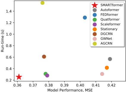
Running Time Efficiency Analysis. As shown in Figure 5, we evaluate SMARTformer with 8 strong baselines, Transformer based models: Autoformer, FEDformer, Quatformer [Chen et al., 2022], Scaleformer[Shabani et al., 2022], Non-stationary Transformers (represented as Stationary) and GNN based models: DGCRN [Li et al., 2021], GWNet [Wu et al., 2019] and AGCRN [Bai et al., 2020]. Experiments are conducted on the Weather Dataset with a 96 length input and a 720 predicted length output. Our SMARTformer is the fastest and best accurate among the 9 models.
5 Conclusion
Long time series forecasting is notably associated with the ability to stably capture local dependencies. Thus, we propose SMARTformer, consisting of three effective mechanisms, where Time-Independent Embedding enhances periodic variations, Integrated Window Attention achieves complementary clues in various receptive fields, and SemiAutoregressive Decoder identifies solid local and global characteristics in two stages. Extensive experiments show that our framework achieves superior forecasting performance.
Ethical Statement
There are no ethical issues.
Acknowledgements
This work was partially supported by the National Key Research and Development Program of China (No. 2018AAA0100204), a key program of fundamental research from Shenzhen Science and Technology Innovation Commission (No. JCYJ20200109113403826), the Major Key Project of PCL (No. 2022ZD0115301), and an Open Research Project of Zhejiang Lab (NO.2022RC0AB04).
@inproceedings{ijcai2023p241,
  title     = {SMARTformer: Semi-Autoregressive Transformer with Efficient Integrated Window Attention for Long Time Series Forecasting},
  author    = {Li, Yiduo and Qi, Shiyi and Li, Zhe and Rao, Zhongwen and Pan, Lujia and Xu, Zenglin},
  booktitle = {Proceedings of the Thirty-Second International Joint Conference on
               Artificial Intelligence, {IJCAI-23}},
  publisher = {International Joint Conferences on Artificial Intelligence Organization},
  editor    = {Edith Elkind},
  pages     = {2169--2177},
  year      = {2023},
  month     = {8},
  note      = {Main Track},
  doi       = {10.24963/ijcai.2023/241},
  url       = {https://doi.org/10.24963/ijcai.2023/241},
}
TY - CPAPER TI - SMARTformer: Semi-Autoregressive Transformer with Efficient Integrated Window Attention for Long Time Series Forecasting AU - Li, Yiduo AU - Qi, Shiyi AU - Li, Zhe AU - Rao, Zhongwen AU - Pan, Lujia AU - Xu, Zenglin T2 - Proceedings of the Thirty-Second International Joint Conference on Artificial Intelligence, IJCAI-23 PB - International Joint Conferences on Artificial Intelligence Organization PY - 2023 SP - 2169 EP - 2177 DO - 10.24963/ijcai.2023/241 UR - https://doi.org/10.24963/ijcai.2023/241 ER -Copied
Machine-readable versions of this paper, for tools and AI agents:





