
GIDnets: Generative Neural Networks for Solving Inverse Design Problems via Latent Space Exploration
Proceedings of the Thirty-Second International Joint Conference on Artificial Intelligence. Main Track. Pages 3404-3413.
https://doi.org/10.24963/ijcai.2023/379
Keywords
- Machine Learning: ML: Experimental methodology
- Machine Learning: ML: Autoencoders
- Machine Learning: ML: Applications
Abstract
In a number of different fields, including Engeneering, Chemistry and Physics, the design of technological tools and device structures is increasingly supported by deep-learning based methods, which provide suggestions on crucial architectural choices based on the properties that these tools and structures should exhibit. The paper proposes a novel architecture, named GIDnet, to address this inverse design problem, which is based on exploring a suitably defined latent space associated with the possible designs. Among its distinguishing features, GIDnet is capable of identifying the most appropriate starting point for the exploration and of likely converging into a point corresponding to a design that is a feasible one. Results of a thorough experimental activity evidence that GIDnet outperforms earlier approaches in the literature.
- [Asano and Noda, 2018] Takashi Asano and Susumu Noda. Optimization of photonic crystal nanocavities based on deep learning. Optics Express, 26(25):32704-32717, 2018.
- [Banerjee et al., 2021] Chaity Banerjee, Chad Lilian, Daniel Reasor, Eduardo Pasiliao, and Tathagata Mukherjee. An application of generative adversarial networks for robust inference in computational fluid dynamics. In Proc. of ICISDM'21, page 74-83, 2021.
- [Chen et al., 2019] Yingshi Chen, Jinfeng Zhu, Yinong Xie, Naixing Feng, and Qing Huo Liu. Smart inverse design of graphene-based photonic metamaterials by an adaptive artificial neural network. Nanoscale, 11(19):9749-9755, 2019.
- [Chiarello et al., 2021] Filippo Chiarello, Paola Belingheri, and Gualtiero Fantoni. Data science for engineering de- sign: State of the art and future directions. Computers in Industry, 129:103447, 2021.
- [Chilwell and Hodgkinson, 1984] John Chilwell and Ian Hodgkinson. Thin-films field-transfer matrix theory of planar multilayer waveguides and reflection from prism- loaded waveguides. Journal of the Optical Society of America, A, 1(7):742-753, 1984.
- [Coli et al., 2022] Gabriele M. Coli, Emanuele Boattini, Laura Filion, and Marjolein Dijkstra. Inverse design of soft materials via a deep learning-based evolutionary strat- egy. Science Advances, 8(3):eabj6731, 2022.
- [Debnath et al., 2021] Arindam Debnath, Adam M Krajew- ski, Hui Sun, Shuang Lin, Marcia Ahn, Wenjie Li, Shan- shank Priya, Jogender Singh, Shunli Shang, Allison M Beese, et al. Generative deep learning as a tool for in- verse design of high entropy refractory alloys. Journal of Materials Informatics, 1(1):3, 2021.
- [Dodaro et al., 2022] Carmine Dodaro, Valeria Fionda, and Gianluigi Greco. LTL on weighted finite traces: Formal foundations and algorithms. In Proc. of IJCAI'22, pages 2606-2612, 2022. IJCAI
- [Glotzer, 2021] Sharon C. Glotzer. Data science for assem- bly engineering. In Proc. of KDD'21, page 2, 2021.
- [Grantham et al., 2022] Karl Grantham, Muhetaer Mukaidaisi, Hsu Kiang Ooi, Mohammad Sajjad Ghaemi, Alain Tchagang, and Yifeng Li. Deep evolutionary learning for molecular design. IEEE Computational Intelligence Magazine, 17(2):14-28, 2022.
- [Greco et al., 2015] Gianluigi Greco, Antonella Guzzo, Francesco Lupia, and Luigi Pontieri. Process discov- ery under precedence constraints. ACM Transactions on Knowledge Discovery from Data, 9(4), 2015.
- [Gómez-Bombarelli et al., 2018] Rafael Gómez- Bombarelli, Jennifer N. Wei, David Duvenaud, José Miguel Hernández-Lobato, Benjamín Sánchez- Lengeling, Dennis Sheberla, Jorge Aguilera-Iparraguirre, Timothy D. Hirzel, Ryan P. Adams, and Alán Aspuru- Guzik. Automatic chemical design using a data-driven continuous representation of molecules. ACS Central Science, 4(2):268-276, 2018. PMID: 29532027.
- [Heyrani Nobari et al., 2021] Amin Heyrani Nobari, Wei Chen, and Faez Ahmed. Pcdgan: A continuous conditional diverse generative adversarial network for inverse design. In Proc. of KDD'21, page 606-616, 2021.
- [Jiang and Fan, 2019] Jiaqi Jiang and Jonathan A. Fan. Global optimization of dielectric metasurfaces using a physics-driven neural network. Nano Letters, 19(8):5366- 5372, 2019.
- [Jiang et al., 2019] Jiaqi Jiang, David Sell, Stephan Hoyer, Jason Hickey, Jianji Yang, and Jonathan A. Fan. Free- form diffractive metagrating design based on generative adversarial networks. ACS Nano, 13(8):8872-8878, 2019.
- [Jiang et al., 2020] Jiaqi Jiang, Mingkun Chen, and Jonathan A. Fan. Deep neural networks for the evalu- ation and design of photonic devices. Nature Reviews Materials, 2020.
- [Kruse et al., 2021] Jakob Kruse, Lynton Ardizzone, Carsten Rother, and Ullrich Köthe. Benchmarking invert- ible architectures on inverse problems. arXiv preprint arXiv:2101.10763, 2021.
- [Lininger et al., 2021] Andrew Lininger, Michael Hinczewski, and Giuseppe Strangi. General inverse design of layered thin-film materials with convolutional neural networks. ACS Photonics, 8(12):3641-3650, 2021.
- [Liu et al., 2018a] Dianjing Liu, Yixuan Tan, Erfan Khoram, and Zongfu Yu. Training deep neural networks for the inverse design of nanophotonic structures. ACS Photonics, 5(4):1365-1369, 2018.
- [Liu et al., 2018b] Zhaocheng Liu, Dayu Zhu, Sean P. Ro- drigues, Kyu-Tae Lee, and Wenshan Cai. Generative model for the inverse design of metasurfaces. Nano Let- ters, 18(10):6570-6576, 2018.
- [Ma et al., 2019] Wei Ma, Feng Cheng, Yihao Xu, Qinlong Wen, and Yongmin Liu. Probabilistic representation and inverse design of metamaterials based on a deep generative model with semi-supervised learning strategy. Advanced Materials, 31(35):1901111, 2019.
- [Mahynski et al., 2020] Nathan A Mahynski, Runfang Mao, Evan Pretti, Vincent K Shen, and Jeetain Mittal. Grand canonical inverse design of multicomponent colloidal crystals. Soft Matter, 16(13):3187-3194, 2020.
- [Mirza and Osindero, 2014] Mehdi Mirza and Simon Osin- dero. Conditional generative adversarial nets. CoRR, abs/1411.1784, 2014.
- [Molesky et al., 2018] Sean Molesky, Zin Lin, Alexander Y Piggott, Weiliang Jin, Jelena Vucković, and Alejandro W Rodriguez. Inverse design in nanophotonics. Nature Pho- tonics, 12(11):659-670, 2018.
- [Nellippallil et al., 2017] Anand Balu Nellippallil, Kevin N Song, Chung-Hyun Goh, Pramod Zagade, BP Gautham, Janet K Allen, and Farrokh Mistree. A goal-oriented, se- quential, inverse design method for the horizontal integra- tion of a multistage hot rod rolling system. Journal of Me- chanical Design, 139(3):031403, 2017.
- [Noh et al., 2020] Juhwan Noh, Geun Ho Gu, Sungwon Kim, and Yousung Jung. Machine-enabled inverse de- sign of inorganic solid materials: promises and challenges. Chemical Science, 11(19):4871-4881, 2020.
- [Peurifoy et al., 2018] John Peurifoy, Yichen Shen, Li Jing, Yi Yang, Fidel Cano-Renteria, Brendan G. DeLacy, John D. Joannopoulos, Max Tegmark, and Marin Soljačić. Nanophotonic particle simulation and inverse design using artificial neural networks. Science Advances, 4(6):eaar4206, 2018.
- [Ren et al., 2020] Simiao Ren, Willie Padilla, and Jordan Malof. Benchmarking deep inverse models over time, and the neural-adjoint method. In H. Larochelle, M. Ranzato, R. Hadsell, M.F. Balcan, and H. Lin, editors, Advances in Neural Information Processing Systems, volume 33, pages 38-48.
- Curran Associates, Inc., 2020.
- [Ren et al., 2022] Simiao Ren, Ashwin Mahendra, Omar Khatib, Yang Deng, Willie J. Padilla, and Jordan M. Malof. Inverse deep learning methods and benchmarks for artificial electromagnetic material design. Nanoscale, 14:3958-3969, 2022.
- [Sekar et al., 2019] Vinothkumar Sekar, Mengqi Zhang, Chang Shu, and Boo Cheong Khoo. Inverse design of airfoil using a deep convolutional neural network. Aiaa Journal, 57(3):993-1003, 2019.
- [Sridharan et al., 2022] Bhuvanesh Sridharan, Manan Goel, and U. Deva Priyakumar. Modern machine learning for tackling inverse problems in chemistry: molecular design to realization. Chemical Comm., 58:5316-5331, 2022.
- [Unni et al., 2021] Rohit Unni, Kan Yao, Xizewen Han, Mingyuan Zhou, and Yuebing Zheng. A mixture-density- based tandem optimization network for on-demand in- verse design of thin-film high reflectors. Nanophotonics, 10(16):4057-4065, 2021.
- [Wiecha et al., 2021] Peter R. Wiecha, Arnaud Arbouet, Christian Girard, and Otto L. Muskens. Deep learning in nano-photonics: inverse design and beyond. Photonic Re- search, 9(5):B182-B200, 2021.
- [Yeung et al., 2021] Christopher Yeung, Ju-Ming Tsai, Brian King, Benjamin Pham, David Ho, Julia Liang, Mark W. Knight, and Aaswath P. Raman. Multiplexed supercell metasurface design and optimization with tandem residual networks. Nanophotonics, 10(3):1133-1143, 2021.
- [Zaabab et al., 1995] A.H. Zaabab, Qi-Jun Zhang, and M. Nakhla. A neural network modeling approach to cir- cuit optimization and statistical design. IEEE Transactions on Microwave Theory and Techniques, 43(6):1349-1358, 1995.
- [Zhang et al., 2018] C. Zhang, J. Jin, W. Na, Q. Zhang, and M. Yu. Multivalued neural network inverse modeling and applications to microwave filters. IEEE Trans. on Mi- crowave Theory and Techniques, 66(8):3781-3797, 2018.
References were extracted automatically from the PDF and may contain errors.
Full text extracted automatically from the PDF; figures, tables and equations may differ. The PDF is the version of record.
1 Introduction
The availability of increasingly effective AI techniques is paving the way to conceive novel approaches for supporting production processes over a wide spectrum of domains (e.g., [Chiarello et al., 2021; Glotzer, 2021; Sridharan et al., 2022; Coli et al., 2022; Debnath et al., 2021]). In particular, in fields such as Engineering, Chemistry and Physics, the design of technological tools and device structures is progressively supported by inverse design (deep learning) methods, providing suggestions on crucial architectural choices based on the properties that these tools and devices should exhibit [Sekar et al., 2019; Nellippallil et al., 2017; Molesky et al., 2018; Noh et al., 2020; Mahynski et al., 2020].
In order to illustrate the idea behind inverse design, let us consider a photonic application scenario where the approach is rapidly increasing its popularity [Wiecha et al., 2021; Jiang et al., 2020]. In this context, the forward problem is easily solved: a number of electromagnetic simulators are already available in the literature which are able to accurately predict the electromagnetic response of any given photonic device structure, such as a metamaterial or a metasurface-see the top part of Figure 1. In practice, however, physicians and optical engineers have to face the inverse problem. Indeed, they would like to design novel structures exhibiting some specific and desired electromagnetic responses; and, to this end, traditionally they have to explore the design space by considering several candidate structures before one enjoying the desired properties is found, possibly guiding the search with their knowledge about previous designs.
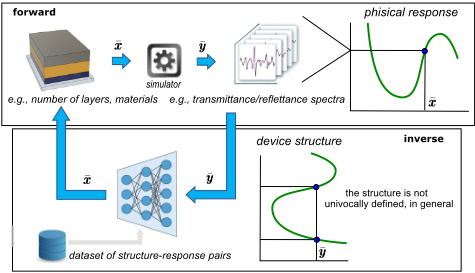
More formally, let S ⊆ Rn be the set of the feasible "input" values (e.g., encodings of the device structures that are allowed). Then, for a given forward function F : S → Rm (e.g., the physical simulator) and desired "output" value ¯ y ∈ Rm (e.g., the desired spectral response), the inverse design problem consists of computing a value ¯ x ∈ S (e.g., the encoding of a device structure) such that ¯ y = F(¯ x). In particular, to accomplish the task, we can exploit the availability of a dataset D = {(xi,yi)}i∈{1,...,q} of (structure-response) pairs such that, for each i ∈ {1, ..., q}, xi ∈ S and yi = F(xi) hold; indeed, D can be built via the simulator or it records results of experiments carried out on real structures.
Clearly enough, deep learning methods can help designers to avoid their time-consuming exploration over S, by using in a systematic way the given dataset D. In fact, we might be tempted to view inverse design as a regression task, where we are asked to end up with a model that is trained to predict xi based on yi, for each i ∈ {1, ..., q}. However, directly learning a model of this kind can be rather challenging in practice, because an "inverse function" is typically not well-defined at all: just think that D often contains several different structures with similar or identical responses (as in Figure 1), so that we are in charge of training a model with contrasting information. In addition, the output of inverse design typically consists of device structures that are one-hot encoded, hence requiring special care to deal with the feasibility of the solutions being produced. Combined with the fact that output spaces are likely high-dimensional, these characteristics pose specific challenges that already elicited the proposal of a number of ad-hoc solution approaches.
The starting point of our work is precisely a review of the most prominent deep-learning based methods proposed in the literature for inverse design. Despite their specific technical differences, most of existing methods share the idea of looking for the solution ¯ x by directly working at the level of the space Rn ; indeed, they have been mainly conceived to deal with applications where Rn is a low-dimensional space. By departing from these approaches, a few works in the literature have already advocated the benefits of mapping the input space into a continuous latent space [G´omez-Bombarelli et al., 2018; Ma et al., 2019]. This perspective is taken in the paper, by proposing a neural network architecture, named GIDNET, where the latent space is additionally constrained to the feasible region S and an exploration algorithm is used to end up with more accurate solutions. The benefits of these two novel ingredients will be eventually evidenced by the results of a thorough experimental activity conducted over several state-of-the-art benchmark datasets arising in different contexts (going beyond photonic applications). 1
2 RelatedWorks
We next classify inverse design methods in two main groups, which we name as output-independent and output-dependent.
Output-independent Methods. Methods in this group are aimed at building an inverse function I : Rm → S such that, for each y ∈ Rm, F(I(y)) = y. So, they work on the entire output space Rm, and do not require any kind of fine-tuning when some specific output value ¯ y ∈ Rm is given to hand and we look for the corresponding input ¯ x such that F(¯ x) = ¯ y.
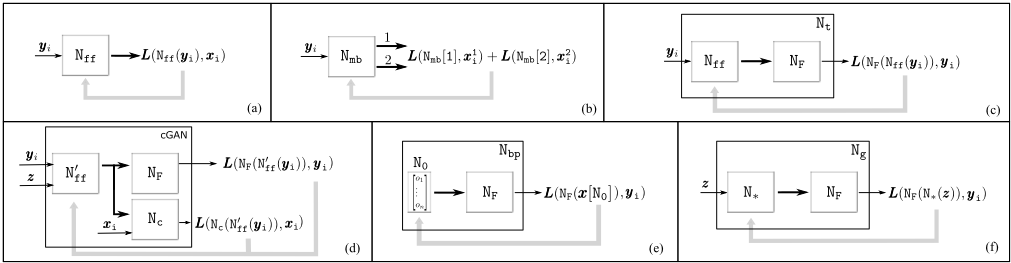
The basic method within this group models the inverse function via a network Nff, which is trained over D = {(xi,yi)}i∈{1,...,q} by receiving as input the values yi and returning as output the estimated inverse Nff(yi), with the loss L to be optimized being its distance from xi-Figure 2(a). In fact, Nff tends to remain improperly trained whenever F is not invertible because several input values can be associated with the same output [Jiang et al., 2020].
1 A more detailed discussion of the experimental settings and results is available in the Supplementary Material.
To overcome this problem, a multi-branched architecture Nmb has been proposed by Zhang et al. (2018). The network receives again yi, by however producing h > 0 outputs, being all possible different inverse values. The weights of Nmb are trained by optimizing the sum of the loss functions over the various outputs-see Figure 2(b), for an illustration with 2 branches. Unfortunately, however, this approach is often unviable in practice [Wiecha et al., 2021], since it requires a datasets storing, for each output value, all corresponding input values (which is an information that we typically lack).
Other approaches use a tandem network Nt [Liu et al., 2018a; Yeung et al., 2021]. The idea is to pre-train a network NF approximating the forward function F. Then, NF is coupled with Nff-see Figure 2(c). As a result, the tandem network acts as an autoencoder; however, the loss function (minimizing the distance between the input and the output of Nt) is optimized via backpropagation over the weights of Nff only; indeed, the pre-trained weights of NF are freezed. After the training, for any value ¯ y, the solution is given by Nff(¯ y ).
A different approach is to modify Nff into a network N′ff receiving as input yi plus some random noise z, and producing xi as output-see Figure 2(d). In fact, the given output value ¯ y can be feed to the network many times, each time together with a different noise value, thereby producing several input values ¯ x associated with ¯ y-so that we can pick the best one. This method also includes a critic/discriminative network Nc enforcing that, on the training input yi and whatever noise z is added, N′ff (yi, z) converges to xi [Liu et al., 2018b; Jiang et al., 2019]. Indeed, the networks Nc and N′ff are eventually trained according to the conditional GAN framework [Mirza and Osindero, 2014; Wiecha et al., 2021].
Output-dependent Methods. Output-dependent methods exploit the knowledge of ¯ y, thereby typically producing results of better quality for their ability to fine tune (on ¯ y) some pre-trained architecture. Noticeable examples are the backpropagation-based methods by [Zaabab et al., 1995; Peurifoy et al., 2018; Asano and Noda, 2018]-see Figure 2(e). The idea is to use the pre-trained network NF coupled with a network N0 with no input, and with one layer only consisting of n nodes whose weights are initialized at random. The network N0 essentially encodes a value in Rn , say x[N0], which is passed to NF. The loss function for the resulting network Nbp is now meant to minimize the distance between ¯ y and NF(x[N0]), and it is optimized by backpropagation over the weighs of N0 only (that is, NF is freezed as usual). Eventually, the desired input value ¯ x (such that ¯ y = F(¯ x)) is given by x[N0] after the updates have been performed. A drawback is that the space of the weights is rather narrow, so that they often end up with undesired local optima [Jiang et al., 2020]. In fact, a more general architecture can be obtained by replacing N0 with the network Nff [Unni et al., 2021]. This leads to an output-dependent version of the tandem network in Figure 2(c)-which we use in the experiments.
A different approach to face that drawback is given by the Neural Adjoint (NA) method [Ren et al., 2020]-which is a variant of the method in Figure 2(e), hereinafter referred to as (e∗ ). For a desired ¯ y, the method repeats T times the optimization of x[N0], by starting from different random initialization of the N0 weights; in addition, it introduces a boundary loss to constrain the final design x[N0] to be a normally distributed variable. Notably, over real-valued inverse design benchmarks, it has been shown that the method achieves comparable or better performances than earlier methods [Ren et al., 2020], including methods based on (cVAE) variational autoencoder architectures whose latent space is conditioned by the knowledge of the output [Ma et al., 2019].
A different generative approach has been proposed by Jiang and Fang (2019). Their architecture (call it Ng) can be seen as a generalization of Nbp, where in place of N0 a more complex network N∗ is used-Figure 2(f). In particular, N∗ takes as input some random noise z and produces a value in Rn , say x[N∗(z)]. For the given output value ¯ y, backpropagation is used to optimize the weights of N∗, by considering as input for the network different samples of a uniformly distributed random variable. The result ¯ x is taken as the value x[N∗(z)] computed during the training and for which the distance between F(x[N∗(z)]) and ¯ y is minimized.
Finally, we mention that a VAE-based variant of the architecture in Figure 2(f) has been proposed too, where N∗ is pre-trained as a decoder of a variational autoencoder and z is sampled from the latent space conditioned on the output and is optimized given ¯ y. Notably, this approach has been specifically designed [G´omez-Bombarelli et al., 2018] to deal with scenarios where the feasible region S ⊆ Rn is associated with a proper one-hot encoding of some categorical features.
Our works shares with [G´omez-Bombarelli et al., 2018] the idea of dealing with an embedding of Rn into a latent space. However, while that work relies on a plain optimization of a random point, we next introduce a method that explores large portions of the latent space to find better solutions, by eventually starting from a meaningful initialization.
3 Description of the GIDNET Approach
To tackle the inverse design problem on a generic function F : S → Rm, with S ⊆ Rn , we propose an output-dependent method where, for any ¯ y ∈ Rm, the desired value ¯ x ∈ Rn such that ¯ y = F(¯ x) is built by means of a generative architecture. Our method founds on the following three ideas:
- First, we embed the space Rn into a suitably-defined latent space Rh , which is relevant to deal with input spaces associated with complex representations going beyond plain numerical values (such as, for instance, with onehot encodings of physical structures).
- Second, we pick a point in the latent space (corresponding to the solution in the input space) via a guided exploration starting from a convenient initial configuration. In particular, we first identify the k pairs (xjℓ , yjℓ ) ∈ D for which the distance between yjℓ and ¯ y is minimized, i.e., we look for the nearest neighbors of ¯ y. Then, we provide the input parts of such pairs (namely, xjℓ ) as starting seeds, and we design an architecture that selects an initial configuration 2 which comes as a linear combination of that seeds. Eventually, the generator is feed with random noise to implement a mechanism that explores the latent space all around that initial configuration.
- Finally, our architecture takes care of dealing with the feasibility constraints that restrict the space Rn to some subset S ⊆ Rn associated with a proper one-hot encoding of the categorical features (e.g., the materials of the device structure). Our solution choice is to deal with that constraints at the embedding, by using an autoencoder architecture that forces each value in the latent spaceeven though associated with an input that has been never seen in the training data-to be mapped into a valid encoding in S. This guarantees that all adjustments to the weights needed to optimize the loss function correspond to a meaningful exploration of the latent space.
In the following, we first detail the neural architecture and then discuss the algorithm to compute ¯ x, given ¯ y.
3.1 Neural Network Architecture
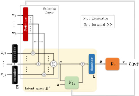
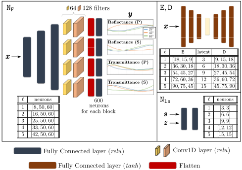
The Generative Inverse Design network (short: GIDNET) we propose to address inverse design is illustrated in Figure 3.
There, we can first notice an encoder E and a decoder D, which allow GIDNET to work on an embedding of Rn into a suitable latent space Rh . In fact, E and D define an autoencoder that is pre-trained over the input-components of D, namely on {xi}i∈{1,...,q}. The autoencoder is a standard one, except for how it handles the categorical features. Indeed, let xi,1, ...,xi,ℓ be the components of xi that one-hot encode some given categorical feature over ℓ alternatives, i.e., such that ∑ℓj=1 xi,j = 1 and xi,j ∈ {0, 1}, for each j ∈ {1, ..., ℓ}. Let x′i,1 = D(E(xi,1)), ...,x′i,ℓ = D(E(xi,ℓ)) be the corresponding values produced by the autoencoder. Then, the last layer of D is defined to be a softmax, so that ∑ℓj=1 x′i,j = 1 and 0 ≤ x′i,j ≤ 1, for each j ∈ {1, ..., ℓ}. In fact, such values might be arbitrary far from Boolean values; for instance, the autoencoder can well produce an output where each value is close to 1/ℓ. To avoid these circumstances, we use the following loss function to train the autoencoder:
2 Different methods (i.e., not necessarily based on the nearest neighbors) can select the starting seeds, leading to different designs that can be further evaluated and selected by the user.
where Γ(x′i,1 , ...,x′i,ℓ ) = -((x′i,1 )2 + · · · + (x′i,ℓ )2 ). In fact, the former term is the reconstruction error, while the latter (whose impact can be tuned via the factor λ0 ≥ 0) is a regularization term leading to configurations where precisely one of the components in {x′i,1 , ...,x′i,ℓ } approaches to 1. The second block that emerges from Figure 3 is a network NF simulating the forward function F. Its weights are trained on D by considering the loss ∑qi=1 ||NF(xi) - yi||2. That is, we would like that the network is capable of predicting the output yi given the input xi. In fact, the use of this network is reminiscent of some of the approaches in Figure 2.
After having discussed E, D and NF, we are now in the position of appreciating the architecture of GIDNET. Note that it receives as input k seeds, say xj1 , ...,xjk . These seeds are then embedded into the h-dimensional latent space via the encoder E : Rn → Rh . Then, a selection layer is used to provide GIDNET with the freedom to pick one of these seeds (or a combination of them); this is achieved by introducing the weights w1, ..., wk, and simply defining:
Intuitively, s defines a good point from which starting the exploration. Indeed, GIDNET includes a conditional generator Nls which takes care of the exploration of the latent space (in the inverse computation phase described below); from the architectural viewpoint, we just note here that it receives as input s plus some random noise z and produces a value Nls(s,z) ∈ Rh . This is used to define the output value that will be returned after decoding via D : Rh → Rn :
Eventually, to check the quality of ¯ x, the architecture uses NF to simulate the given forward function F (i.e., y = NF(¯ x)).
3.2 Inverse Computation
After E, D, and NF have been trained over D, we freeze their weights. Hence, in the inverse computation phase, the trainable weights are w1, .., wk plus all weights of the conditional generator Nls. These weights are re-initialized and re-trained each time an output value ¯ y is given and we look for an input ¯ x such that ¯ y = F(¯ x). The algorithm is next discussed.
First, we have to compute the k seeds xj1 , ...,xjk . To this end, we define xj1 as 0 ∈ Rn (that is, we allow GIDNET to neutralize the seeds), and we take xj2 , ...,xjk from the pairs in D, i.e., {(xj2 ,yj2 ), ..., (xjk ,yjk )} ⊆ D, in a way that there is no pair (xi,yi) ∈ D such that ||yi - ¯ y||2 < maxi∈{2,...k} ||yjk - ¯ y||2; in words, we take the k-1 points whose corresponding forward values are the closest to ¯ y over all pairs in D-ties are resolved at random.
In fact, the seeds are just constant values that initialize the starting point s according to Equation (2). Concerning the trainable weights, instead, we initialize Nls at random while we take wi = 1/k, for each i ∈ {1, ...k}, thereby starting the exploration from the centroid of the k seeds.
Given this initial configuration, we then train GIDNET via a number of training steps where ¯ y is fixed and where different samples z from a uniform distribution are given as input to the conditional generator Nls. Intuitively, by starting from the seed s, each time a different value z is feed to the network, we aim at adjusting the weights of the conditional generator to end up with an output value y that gets even closer to ¯ y. Therefore, the sequence of the training steps corresponds to a path in the latent space leading to a point that is a good solution. In fact, we define the loss function L(y, ¯ y ):
where Γ(w1, ..., wk) = - (w2 1 + · · · +w2 k ) is the same regularization function used for training E and D, and where the term ε(x) = ||D(E(x)) -x||2 is aimed at minimizing the reconstruction error of the autoencoder on input x.
Eventually, w1, ...,wk and the weights in Nls are updated by minimizing the loss L(y, ¯ y). Hence, we explore the latent space while allowing GIDNET to select a different initial configuration s. The value x that is returned as output by GIDNET is the one computed via Equation (3) during the training phase, and for which the distance between NF(x) and ¯ y is minimized. Furthermore, given that the blocks E, D, and NF are trained independently on the number k of seeds, it makes sense to re-execute the inverse computation step over different subsets of seeds by taking the best result obtained over the various configurations. By doing so, we enlarge the portion of the latent space that is explored. Similarly, we re-execute the inverse computation step by changing the learning rates and taking the best results derived over them.
4 Experiments
To shed lights on the behaviour of GIDNET, we next discuss the results of a thorough experimental activity, where we considered all methods discussed in Section 2, except the multi-branched approach which-as already mentionedis often unviable in practice. All network architectures we implemented have been instantiated by means of a modelselection phase, based on a gridsearch approach over the hyperparameter space of the network topologies, the learning rates in the stochastic gradient descent algorithm, the initialization strategies, and the kernel constraints. For GIDNET as well as for the other output-dependent methods, in the inverse computation phase, given the value ¯ y, we considered different learning rates in {0.01, 0.05, 0.1, 0.5} to compute ¯ x such that ¯ y = F(¯ x), by taking the best result over them.
| Name | Dim(x) | Dim(y) | Source | |
|---|---|---|---|---|
| Di | fi | 3 | 2 | [here] |
| D5 | Ballistics | 4 | 1 | [Kruse et al., 2021] |
| D6 | Robotic arm | 4 | 2 | [Kruse et al., 2021] |
| D7 | Sine Wave | 2 | 1 | [Ren et al., 2020] |
| D8 | Multilayer Stacks | 5 | 256 | [Chen et al., 2019] |
4.1 GIDNET on Real-Valued Functions
We first discuss the results on the datasets listed in Table 1, which are all defined on real-valued input spaces.
Datasets D1, ...,D4 are novel in the literature: each one comprises 10.000 pairs (xi ∈ R3 ,yi ∈ R2 ) defined via classical functions emerging in physical systems and stressing the absence of a univocally-defined inverse value. For each dataset, we used 7.000 samples for training and 2.900 for validation during training; seed computation for GIDNET was carried out over these 9.900 samples. The remaining 100 samples were, instead, used for assessing the value of the metrics after the training phase has been completed. In particular, we consider L2-norm, MAE and RMSE.
A summary of our findings over D1, ...,D4 is reported in Table 2, from which the improvements provided by GIDNET over earlier methods clearly emerge. The figure also evidences the impact of varying the number k of seeds and of disabling the module Nls implementing the conditional generation approach. The ablation study on k confirms the intuition that it make sense to enlarge the latent space to be explored by considering the best results over different number of seeds; in fact, it also emerges a trend of improvement at the growing of k. Moreover, it emerges that Nls has a strong positive impact on the quality of the results; in fact, it is responsible of the exploration in the latent space (cf. Equation 3). And, finally, it is interesting to observe that GIDNET is rather robust w.r.t. statistical fluctuations over the different samples.
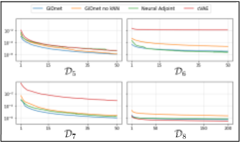
Datasets D5, ...,D8 instead appeared in earlier works and have been extensively used to benchmark earlier methods. Over them, the Neural Adjoint method (e∗ ) emerged as the state of the art, together (in some cases) with the cVAE approach [Ren et al., 2020; Ren et al., 2022; Kruse et al., 2021]. Accordingly, our experiments have been focused on assessing the performances GIDNET in comparison with them (by precisely adopting their experimental setting). Moreover, we also conducted an ablation study by selecting random initializations k seeds, rather than by taking the k nearest neighbors. Results are illustrated in Figure 4, which evidences the good performances of GIDNET even on these settings where the use of the latent space is trivialized by the low dimensionality of the input spaces; moreover, the ablation study further confirms the benefits of appropriately picking the k seeds.
4.2 GIDNET on Categorical Attributes
To assess the behaviour of GIDNET on a function involving categorical attributes, we considered a photonic scenario proposed by Lininger et al. (2021), where the goal is to build a thin-film structure that gives rise to some desired reflectance/transmittance spectra.
Dataset Description. Each structure is made of up to 5 layers, each with thickness within the range [1, 60]nm and whose material can be Ag, Al2O3, ITO, Ni, or TiO2. The input space is therefore Rℓ×(1+5) , with ℓ being the number of layers-indeed, for each layer, we have to represent its thickness plus the material as a one-hot encoding over 5 alternatives. Each structure is associated with reflectance and transmittance spectra, obtained via the transfer matrix method [Chilwell and Hodgkinson, 1984], for two polarizations, at the incident angles of 25, 45, and 65 degrees, for 200 equally spaced points over the range [450, 950]nm and with values in [0, 1]. Thus, the output space is R2×2×3×200 .
For each ℓ ∈ {1, .., 5}, we use 106.820 samples for training, 45.780 samples for validation, and 2.000 samples for computing the metric. The seeds needed by GIDNET are, as usual, computed over the traning and validation samples.
For a closer look at the dataset of Lininger et al. (2021), note that about 5% of the samples have very similar spectra, with a significant portion of them being associated to structures different from each other.The absence of clearly defined inverse values on these samples is congenial to stress the capabilities of inverse design approaches.
ComparedMethods andMetric. The GIDNET configurations resulting from the model-selection phase are reported in Figure 5. During the inverse computation step, GIDNET explores a space with k ∈ {3, 6, 9, 12, 18, 30, 50} and learning rates in {0.01, 0.05, 0.1, 0.5}, by taking the best results achieved over them. A similar exploration over the learning rates has been implemented for the other outputdependent methods being tested. Performances of the methods have been compared via the spectral root mean squared error [Lininger et al., 2021], srmse for short, between the spectra (in R2×2×3×200 ) associated to the metamaterial designed by the methods and the actual ones.
| Other methods | GIDNET | ||||||||||
|---|---|---|---|---|---|---|---|---|---|---|---|
| (a) | (c) | (d) | (e*) | (f) | k=12 | k=7 | k=5 | k=3 | k=1 | no Nls | |
| L2 | 0.030 (±0.022) | 0.155 (±0.570) | 0.018 (±0.012) | 0.004 (±0.0256) | 0.112 (±0.286) | 0.005 (±0.005) | 0.005 (±0.007) | 0.004 (±0.004) | 0.005(±0.006) | 0.083 (±0.304) | 0.040 (±0.021) |
| D1 MAE | 0.019 (±0.015) | 0.092 (±0.343) | 0.012 (±0.009) | 0.002 (±0.0166) | 0.068 (±0.172) | 0.003 (±0.003) | 0.003 (±0.005) | 0.003 (±0.003) | 0.003 (±0.004) | 0.055 (±0.198) | 0.026 (±0.014) |
| RMSE | 0.037 | 0.590 | 0.022 | 0.0259 | 0.307 | 0.006 | 0.009 | 0.006 | 0.007 | 0.315 | 0.045 |
| L2 | 0.009 (±0.011) | 0.007 (±0.012) | 0.017 (±0.022) | 0.007 (±0.0392) | 0.009 (±0.014) | 0.005 (±0.003) | 0.006 (±0.005) | 0.006 (±0.005) | 0.006 (±0.008) | 0.029 (±0.059) | 0.054 (±0.023) |
| D2 MAE | 0.006 (±0.008) | 0.005 (±0.009) | 0.011 (±0.015) | 0.004 (±0.0224) | 0.006 (±0.009) | 0.003 (±0.002) | 0.004 (±0.003) | 0.004 (±0.004) | 0.004 (±0.005) | 0.020 (±0.039) | 0.035 (±0.015) |
| RMSE | 0.014 | 0.014 | 0.028 | 0.040 | 0.016 | 0.006 | 0.008 | 0.008 | 0.010 | 0.066 | 0.059 |
| L2 | 0.010 (±0.021) | 0.026 (±0.07) | 0.009 (±0.023) | 0.016 (±0.073) | 0.022 (±0.051) | 0.006 (±0.020) | 0.005 (±0.019) | 0.005 (±0.019) | 0.005 (±0.019) | 0.033 (±0.116) | 0.029 (±0.032) |
| D3 MAE | 0.006 (±0.012) | 0.015 (±0.04) | 0.005 (±0.013) | 0.0094 (±0.0417) | 0.013 (±0.029) | 0.003 (±0.011) | 0.003 (±0.011) | 0.003 (±0.011) | 0.003 (±0.011) | 0.022 (±0.079) | 0.018 (±0.018) |
| RMSE | 0.023 | 0.075 | 0.025 | 0.0745 | 0.056 | 0.020 | 0.019 | 0.019 | 0.019 | 0.121 | 0.043 |
| L2 | 0.012 (±0.013) | 0.006 (±0.015) | 0.024 (±0.029) | 0.0012 (±0.0057) | 0.007 (±0.015) | 0.005 (±0.014) | 0.013 (±0.047) | 0.012 (±0.049) | 0.021 (±0.064) | 0.586 (±0.688) | 0.035 (±0.043) |
| D4 MAE | 0.008 (±0.008) | 0.004 (±0.011) | 0.016 (±0.020) | 0.0007 (±0.0032) | 0.005 (±0.010) | 0.003 (±0.009) | 0.008 (±0.031) | 0.008 (±0.032) | 0.014 (±0.043) | 0.395 (±0.482) | 0.023 (±0.030) |
| RMSE | 0.017 | 0.016 | 0.038 | 0.0059 | 0.016 | 0.014 | 0.048 | 0.051 | 0.067 | 0.903 | 0.055 |
| ℓ | 3 | 4 | 5 |
|---|---|---|---|
| GIDNET | 0.009 (±0.024) | 0.009 (±0.022) | 0.011 (±0.022) |
| GIDNET no Nls | 0.060 (±0.099) | 0.046 (±0.072) | 0.043 (±0.064) |
In particular, to take care of the feasibility of the solutions, if ¯ x are the values returned by the tested methods, then we first pre-process them by suitably rounding the components associated to the one-hot encodings of the materials over the various layers. Subsequently, for the resulting values (in fact, correctly encoding some device structures), we use the physical simulator at hand [Chilwell and Hodgkinson, 1984] to compute their associated spectra, and the quality of the results (srmse) is eventually assessed over them.
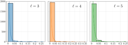
Figure 7: Histograms of srmse for GIDNET, in the photonic scenario, for different number ℓ of material layers.
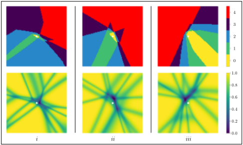
A Look at the Latent Space. As the crucial ingredient of GIDNET is its ability to work at the level of a suitably defined latent space, we took a closer look at it in Figure 6 by considering a sample taken from the dataset with ℓ = 4 layers. In particular, the plots in Figure 6 are centered in the initial point of the exploration defined by GIDNET (with k = 3); then, the three settings (i, ii, and iii) in the figure correspond to an exploration of the latent space over an interval of that point defined by moving along two different dimensions and by fixing all remaining ones. For each setting, the top part reports the number of materials that change compared to the configuration in the initial point, while those at the bottom report the average squared Euclidean norm of the encoding associated with the materials over the various layers. Note that the latent space changes all (4) materials in the region, and that the encoding is always very close to a true one-hot encoding (with a squared Euclidean norm rather close to 1), except in the tiny regions associated with the frontiers of different configurations of the materials (where the squared Euclidean norm approaches to 0).
| ℓ | (a) | (c) | (d) | (e*) | (f) | Liniger et al. | GIDNET | λ0 = 0 | |
|---|---|---|---|---|---|---|---|---|---|
| 1 | srmse | 0.007 (±0.008) | 0.062 (±0.09) | 0.132 (±0.21) | 0.033 (±0.054) | 0.132 (±0.21) | 0.009 | 0.006 (±0.031) | 0.019 (±0.051) |
| one-hot | 0.924 (±0.527) | 0.236 (±0.023) | 0.798 (±0.335) | 0.302 (±0.114) | 0.798 (±0.335) | - | 0.999 (±0.017) | 0.275 (±0.012) | |
| 2 | srmse | 0.010 (±0.012) | 0.098 (±0.117) | 0.117 (±0.133) | 0.049 (±0.050) | 0.117 (±0.133) | 0.007 | 0.008 (±0.032) | 0.077 (± 0.057) |
| one-hot | 0.921 (±0.567) | 0.233 (±0.020) | 0.353 (±0.139) | 0.261 (±0.035) | 0.353 (±0.139) | - | 0.992 (±0.037) | 0.396 (±0.075) | |
| 3 | srmse | 0.015 (±0.032) | 0.084 (±0.104) | 0.031 (±0.034) | 0.059 (±0.053) | 0.083 (±0.09) | 0.016 | 0.009 (±0.024) | 0.052 (± 0.047) |
| one-hot | 0.902 (±0.563) | 0.225 (±0.022) | 0.235 (±0.013) | 0.249 (±0.017) | 0.230 (±0.065) | - | 0.974 (±0.053) | 0.321 (±0.048) | |
| 4 | srmse | 0.038 (±0.162) | 0.078 (±0.100) | 0.042 (±0.043) | 0.061 (±0.051) | 0.078 (±0.081) | 0.127 | 0.009 (±0.022) | 0.057 (± 0.040) |
| one-hot | 0.825 (±0.538) | 0.226 (±0.021) | 0.220 (±0.009) | 0.250 (±0.016) | 0.232 (±0.068) | - | 0.940 (±0.068) | 0.433 (±0.077) | |
| 5 | srmse | 0.050 (±0.087) | 0.053 (±0.065) | 0.050 (±0.054) | 0.059 (±0.053) | 0.069 (±0.071) | 0.095 | 0.011 (±0.022) | 0.047 (±0.056) |
| one-hot | 0.663 (±0.267) | 0.229 (±0.019) | 0.222 (±0.010) | 0.251 (±0.013) | 0.232 (±0.067) | - | 0.911 (±0.082) | 0.647 (±0.145) | |
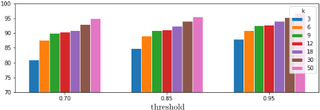
A Look at the Selection Layers. The other crucial ingredient of GIDNET is the use of k seeds to define an appropriate initial configuration for the exploration (cf. s in Equation (3)). Figure 8 illustrates the behaviour of the selection layer in terms of the percentage of samples for which it converges into a linear combination of the seeds-formally, in the inverse computation phase, no weight associated with some seed gets a value greater than the reported threshold. In some cases, GIDNET converges on some specific seed; but, in many cases, it retains the ability to explore a large portion of the search space by converging into a proper linear combination of the seeds; hence, the selection layer cannot be replaced by an approach that iterates over the seeds, by considering each of them as a fixed initial configuration for the exploration. Moreover, note that the higher is the number k of seeds, the more probable is converging to a proper linear combination rather than just to a specific seed.
ALook at the Conditional Generator. Finally, the last architectural component of interest is the conditional generator Nls. The significance of its role can be appreciated by looking at Table 3, where the performances of GIDNET are shown depending on whether the module is enabled. In particular, without Nls, GIDNET lacks the ability of searching over the latent space and it conceptually reduces to optimizing a random point (as in [G´omez-Bombarelli et al., 2018]).
| ℓ | ⋆ | GIDNET | GIDNET no kNN | |
|---|---|---|---|---|
| 3 | srmse | 0.044 (±0.051) | 0.009 (±0.024) | 0.024 (±0.035) |
| one-hot | 0.248 (±0.005) | 0.974 (±0.053) | 0.926 (±0.083) | |
| 4 | srmse | 0.109 (±0.122) | 0.009 (±0.022) | 0.052 (±0.059) |
| one-hot | 0.229 (±0.01) | 0.940 (±0.068) | 0.953 (±0.0643) | |
| 5 | srmse | 0.058 (±0.059) | 0.011 (±0.022) | 0.028 (±0.042) |
| one-hot | 0.205 (±0.004) | 0.911 (±0.082) | 0.964 (±0.047) | |
| ℓ | (c) | (e) | (f) | GIDNET |
|---|---|---|---|---|
| 1 | 8.976 (±0.297) | 2.510 (±0.097) | 7.621 (±0.113) | 7.191 (±0.332) |
| 2 | 8.876 (±0.151) | 2.466 (±0.079) | 7.639 (±0.111) | 7.605 (±0.263) |
| 3 | 8.809 (±0.199) | 2.504 (±0.103) | 7.728 (±0.099) | 7.841 (±0.334) |
| 4 | 13.01 (±0.185) | 2.549 (±0.122) | 7.588 (±0.103) | 7.916 (±0.255) |
| 5 | 16.16 (±0.198) | 2.490 (±0.093) | 7.707 (±0.089) | 8.074 (±0.175) |
Performances. Let us first consider Figure 7 reporting the histograms of the srmse for ℓ ∈ {3, 4, 5}. It emerges that GIDNET is capable of designing metamaterials whose spectral responses are quite close to the desired ones; errors are rather small in general, and negligible in most of the cases. Moreover, there is a trend of (very mild) deterioration in the performances at the growing of the complexity (in terms of number of layers) of the space to be explored by GIDNET.
A summary of the results comparing GIDNET with earlier approaches is then reported in Table 4-for the domain specific method, we report the results that are published by the authors. Note that GIDNET produces solutions with very low srmse, and improvements are significant given that spectra values are in [0, 1]. In particular, note that the cases ℓ ∈ {1, 2} are solved efficiently by all methods, while significant differences emerge on ℓ ∈ {3, 4, 5}, that is, at the growing of the complexity of the underlying search space. Eventually, the summary also reports the feasibly of the solutions in terms of the quality of the one-hot encodings (prior that the results are rounded and adjusted for computing the associated spectra), which confirms the intuition we have derived from Figure 6.
And, finally, it also evidences the significant impact of the strategy we implemented in the autoencoder to deal with the categorical features (cf. λ0 = 0 in Equation (1)). Indeed, by loosing the ability to map the latent space into feasible designs, performances of GIDNET rapidly deteriorates.
In addition to the methods reported in Table 4, we also assessed the performances of the method proposed by [G´omezBombarelli et al., 2018] (and implemented by fine-tuning the building blocks trained for GIDNET), which has been indeed specifically conceived to deal with categorical attributes. That methods works at the level of the latent space (see Section 2), but lacks of a mechanism to explore that space starting from a meaningful initialization. Results in Table 5 confirm that the exploration of GIDNET is crucial to achieve higher levels of performance and, as in Figure 4, they further confirm the benefits of picking k nearest neighbors for the initialization compared to a random initialization (column "no kNN").
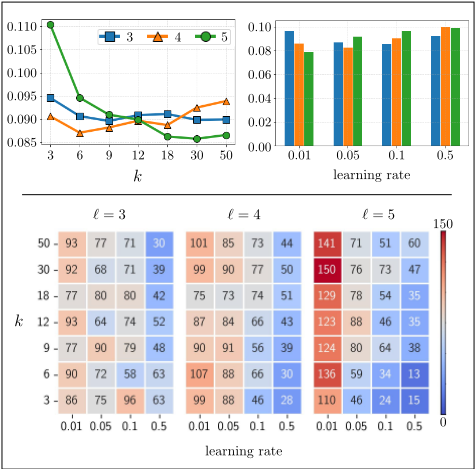
The impact of the number k of seeds and of the learning rates is then analyzed in Figure 9. Observe that increasing the number of seeds as well as reducing the learning rate lead to better performances; in particular, this emerges more clearly over the most complex scenario with ℓ = 5.
Finally, we shed lights on the time requirements, by conducting comparative experiments, on the same phyton environment, over an Intel(R) Xeon(R) Processor E5-2670 v3 (2.30GHz), 24 cores single thread and 96GB of RAMfor training the architectures (before inverse computation), we also use an NVIDIA 2080 GPU. In fact, GIDNET is an output-dependent method, which requires some computational efforts on every structure that has to be designed. While this is hardly relevant in practical design applications (unless timings make the approach unviable), for the sake of completeness, we report in Table 6 such information for GIDNET and all other output-dependent methods.
5 Conclusions and Discussion
We have proposed a deep-learning architecture improving on the performance of existing methods by addressing inverse design by means of a guided exploration of the latent space. In fact, it is known that search-based approaches are effective in domains where the space of the parameters is rather narrow, but they are outperformed by deep learning methods over high dimensional spaces. An interesting avenue of research is, therefore, to define an hybrid method where GIDNET is coupled with a genetic algorithm to explore the search space (in the spirit, e.g.,of [Grantham et al., 2022]).
Similarly, it would be interesting to couple GIDNET with logic-based reasoning engines, in settings where inverse design amounts at looking for the (truth) value of some variables that will eventually lead to satisfy some desired logical goal; in particular, we are interested in considering cost-based settings [Dodaro et al., 2022] and precedence constraints to express temporal properties [Greco et al., 2015].
We conclude by noticing that a different-though relatedproblem is sometimes addressed in the context of inverse design, consisting of learning distributions of existing designs in order to synthesize new designs via sampling (e.g. [Heyrani Nobari et al., 2021; Banerjee et al., 2021]). In this case, we do not a-priori enforce complex properties such as the spectral responses; however, conditioning methods can be used to enforce that samples meet some scalar requirement, such as a performance metric. A natural avenue of further research is, therefore, to assess whether GIDNET can be adapted to effectively address this related problem too.
Ethical Statement
There are no ethical issues.
Acknowledgments
The research reported in the paper was partially supported by the PNRR projects "FAIR (PE00000013) - Spoke 9" and "Tech4You (ECS00000009) - Spoke 6", under the NRRP MUR program funded by the NextGenerationEU.
@inproceedings{ijcai2023p379,
  title     = {GIDnets: Generative Neural Networks for Solving Inverse Design Problems via Latent Space Exploration},
  author    = {Adornetto, Carlo and Greco, Gianluigi},
  booktitle = {Proceedings of the Thirty-Second International Joint Conference on
               Artificial Intelligence, {IJCAI-23}},
  publisher = {International Joint Conferences on Artificial Intelligence Organization},
  editor    = {Edith Elkind},
  pages     = {3404--3413},
  year      = {2023},
  month     = {8},
  note      = {Main Track},
  doi       = {10.24963/ijcai.2023/379},
  url       = {https://doi.org/10.24963/ijcai.2023/379},
}
TY - CPAPER TI - GIDnets: Generative Neural Networks for Solving Inverse Design Problems via Latent Space Exploration AU - Adornetto, Carlo AU - Greco, Gianluigi T2 - Proceedings of the Thirty-Second International Joint Conference on Artificial Intelligence, IJCAI-23 PB - International Joint Conferences on Artificial Intelligence Organization PY - 2023 SP - 3404 EP - 3413 DO - 10.24963/ijcai.2023/379 UR - https://doi.org/10.24963/ijcai.2023/379 ER -Copied
Machine-readable versions of this paper, for tools and AI agents:





