
Computing Abductive Explanations for Boosted Regression Trees
Proceedings of the Thirty-Second International Joint Conference on Artificial Intelligence. Main Track. Pages 3432-3441.
https://doi.org/10.24963/ijcai.2023/382
Keywords
- Machine Learning: ML: Explainable/Interpretable machine learning
- Constraint Satisfaction and Optimization: CSO: Constraint programming
- Machine Learning: ML: Regression
Abstract
We present two algorithms for generating (resp. evaluating) abductive explanations for boosted regression trees. Given an instance x and an interval I containing its value F (x) for the boosted regression tree F at hand, the generation algorithm returns a (most general) term t over the Boolean conditions in F such that every instance x′ satisfying t is such that F (x′ ) ∈ I. The evaluation algorithm tackles the corresponding inverse problem: given F , x and a term t over the Boolean conditions in F such that t covers x, find the least interval I_t such that for every instance x′ covered by t we have F (x′ ) ∈ I_t . Experiments on various datasets show that the two algorithms are practical enough to be used for generating (resp. evaluating) abductive explanations for boosted regression trees based on a large number of Boolean conditions.
- [Adadi and Berrada, 2018] A. Adadi and M. Berrada. Peek- ing inside the black-box: A survey on explainable artificial intelligence (XAI). IEEE Access, 6:52138-52160, 2018.
- [Arrieta et al., 2020] A. Barredo Arrieta, N. Díaz R., J. Del Ser, A. Bennetot, S. Tabik, A. Barbado, S. García, S. Gil- Lopez, D. Molina, R. Benjamins, R. Chatila, and F. Her- rera. Explainable artificial intelligence (XAI): concepts, taxonomies, opportunities and challenges toward respon- sible AI. Inf. Fusion, 58:82-115, 2020.
- [Audemard et al., 2022] G. Audemard, S. Bellart, L. Bounia, F. Koriche, J.-M. Lagniez, and P. Marquis. Trading com- plexity for sparsity in random forest explanations. In Proc. of AAAI'22, pages 5461-5469, 2022.
- [Audemard et al., 2023] G. Audemard, J.-M. Lagniez, P. Marquis, and N. Szczepanski. Computing abductive explanations for boosted trees. In Proc. of the 26th International Conference on Artificial Intelligence and Statistics, AISTATS'23, volume 206 of Proce. of Machine Learning Research, pages 4699-4711, 2023.
- [Barber et al., 2021] Rina Foygel Barber, Emmanuel J. Candès, Aaditya Ramdas, and Ryan J. Tibshirani. Predic- tive inference with the jackknife+. The Annals of Statistics, 49(1):486-507, 2021.
- [Caruana et al., 2020] R. Caruana, S. M. Lundberg, M. Túlio Ribeiro, H. Nori, and S. Jenkins. Intelligible and explain- able machine learning: Best practices and practical chal- lenges. In Proc. of KDD'20, pages 3511-3512. ACM, 2020.
- [Chen and Guestrin, 2016] T. Chen and C. Guestrin. XG- Boost: A scalable tree boosting system. In Proc. of KDD'16, page 785-794, 2016.
- [Choi et al., 2020] A. Choi, A. Shih, A. Goyanka, and A. Darwiche. On symbolically encoding the behavior of random forests. In Proc. of FoMLAS'20, 3rd Workshop on Formal Methods for ML-Enabled Autonomous Systems, Workshop at CAV'20, 2020.
- [Cplex, 2009] IBM ILOG Cplex. V12. 1: User's manual for cplex. International Business Machines Corporation, 46(53):157, 2009.
- [Cui et al., 2015] Z. Cui, W. Chen, Y. He, and Y. Chen. Opti- mal action extraction for random forests and boosted trees. In Proc. of KDD'15, pages 179-188, 2015.
- [Darwiche and Hirth, 2020] A. Darwiche and A. Hirth. On the reasons behind decisions. In Proc. of ECAI'20, pages 712-720, 2020.
- [Doshi-Velez and Kim, 2017] F. Doshi-Velez and B. Kim. A roadmap for a rigorous science of interpretability. CoRR, abs/1702.08608, 2017.
- [Even et al., 1976] S. Even, A. Itai, and A. Shamir. On the complexity of timetable and multicommodity flow prob- lems. SIAM J. Comput., 5(4):691-703, 1976.
- [Gorji and Rubin, 2022] N. Gorji and S. Rubin. Sufficient reasons for classifier decisions in the presence of domain constraints. In Proc. of AAAI'22, pages 5660-5667, 2022.
- [Hada and Carreira-Perpiñán, 2021] S.S. Hada and M. Carreira-Perpiñán. Exploring counterfactual ex- planations for classification and regression trees. In Joint European Conference on Machine Learning and Knowledge Discovery in Databases, pages 489-504, 2021.
- [Ignatiev et al., 2019a] A. Ignatiev, N. Narodytska, and J. Marques-Silva. Abduction-based explanations for ma- chine learning models. In Proc. of AAAI'19, pages 1511- 1519, 2019.
- [Ignatiev et al., 2019b] A. Ignatiev, N. Narodytska, and J. Marques-Silva. On validating, repairing and refining heuristic ML explanations. CoRR, abs/1907.02509, 2019.
- [Ignatiev et al., 2022] A. Ignatiev, Y. Izza, P.J. Stuckey, and J. Marques-Silva. Using MaxSAT for efficient explana- tions of tree ensembles. In Proc. of AAAI'22, pages 3776- 3785, 2022.
- [Ignatiev, 2020] A. Ignatiev. Towards trustable explainable AI. In Proc. of IJCAI'20, pages 5154-5158, 2020. IJCAI
- [Izza and Marques-Silva, 2021] Y. Izza and J. Marques- Silva. On explaining random forests with SAT. In Proc. of IJCAI'21, pages 2584-2591, 2021. IJCAI
- [Kanamori et al., 2020] K. Kanamori, T. Takagi, K. Kobayashi, and H. Arimura. DACE: distribution- aware counterfactual explanation by mixed-integer linear optimization. In Proc. of IJCAI'20, pages 2855-2862, 2020.
- [Ke et al., 2017] G. Ke, Q. Meng, Th. Finley, T. Wang, W. Chen, W. Ma, Q. Ye, and T. Liu. Lightgbm: A highly efficient gradient boosting decision tree. In Proc. of NeurIPS'17, pages 3146-3154, 2017.
- [Koenker, 2005] R. Koenker. Quantile Regression. Econo- metric Society Monographs. Cambridge University Press, 2005.
- [Kontokosta, 2019] S. Papadopoulosand C. Kontokosta. Grading buildings on energy performance using city benchmarking data. Applied Energy, 233:244-253, 2019.
- [Letzgus et al., 2022] S. Letzgus, P. Wagner, J. Lederer, W. Samek, K.R. Müller, and G. Montavon. Toward ex- plainable artificial intelligence for regression models: A methodological perspective. IEEE Signal Process. Mag., 39(4):40-58, 2022.
- [Ling and Kenny, 1981] R. Ling and D. Kenny. Correlation and causation. Journal of the American Statistical Associ- ation, 77:489, 1981.
- [Lipton, 2018] Z. C. Lipton. The mythos of model inter- pretability. Communications of the ACM, 61(10):36-43, 2018.
- [Marques-Silva and Ignatiev, 2022] J. Marques-Silva and A. Ignatiev. Delivering trustworthy AI through formal XAI. In Proc. of AAAI'22, pages 12342-12350, 2022.
- [Miller, 2019] T. Miller. Explanation in artificial intelli- gence: Insights from the social sciences. Artificial Intel- ligence, 267:1-38, 2019.
- [Molnar, 2019] Ch. Molnar. Interpretable Machine Learn- ing -A Guide for Making Black Box Models Explainable. Leanpub, 2019.
- [Moore and Bell, 2022] A. Moore and M. Bell. XGBoost, a novel explainable AI technique, in the prediction of my- ocardial infarction, a UK biobank cohort study. medRxiv, 2022.
- [Narayanan et al., 2018] M. Narayanan, E. Chen, J. He, B. Kim, S. Gershman, and F. Doshi-Velez. How do hu- mans understand explanations from machine learning sys- tems? an evaluation of the human-interpretability of expla- nation. CoRR, abs/1802.00682, 2018.
- [Parmentier and Vidal, 2021] A. Parmentier and T. Vidal. Optimal counterfactual explanations in tree ensembles. In Proc. of ICML'21, volume 139 of Proceedings of Machine Learning Research, 2021.
- [Rudin et al., 2021] C. Rudin, C. Chen, Z. Chen, H. Huang, L. Semenova, and C. Zhong. Interpretable machine learn- ing: Fundamental principles and 10 grand challenges. CoRR, abs/2103.11251, 2021.
- [Shih et al., 2018] A. Shih, A. Choi, and A. Darwiche. A symbolic approach to explaining bayesian network classi- fiers. In Proc. of IJCAI'18, pages 5103-5111, 2018. IJCAI
- [Strumbelj and Kononenko, 2011] E. Strumbelj and I. Kononenko. A general method for visualizing and explaining black-box regression models. In Adaptive and Natural Computing Algorithms ICANNGA, volume 6594 of LNCS, pages 21-30, 2011.
- [Xu et al., 2019] F. Xu, H. Uszkoreit, Y. Du, W. Fan, D. Zhao, and J. Zhu. Explainable AI: A brief survey on his- tory, research areas, approaches and challenges. In Proc. of NLPCC'19, pages 563-574, 2019.
References were extracted automatically from the PDF and may contain errors.
Full text extracted automatically from the PDF; figures, tables and equations may differ. The PDF is the version of record.
1 Introduction
The past few years have witnessed the quick development of a new field, called eXplainable AI (XAI), aroused by the large spectrum of applications leveraging the stunning predictive power of machine learning (ML) models, their opacity, and the tremendous need for gaining trust in such models, especially when they are used in safety-critical applications (see for instance [Doshi-Velez and Kim, 2017; Adadi and Berrada, 2018; Lipton, 2018; Molnar, 2019; Xu et al., 2019; Arrieta et al., 2020; Caruana et al., 2020; Rudin et al., 2021]).
So far, most works about XAI have been concerned with explanation and verification issues about classification functions, i.e., mappings from the set X of instances to a finite set C of classes. In contrast, in this paper, we consider the generation and the evaluation of explanations for regression functions, i.e., mappings from X to R. The explanations sought are abductive ones, i.e., they are intended to explain why the instances x ∈ X that are considered have been mapped to their corresponding values f(x) by the regression function f. In the following, we focus on regression functions given by boosted regression trees, that are combinatorial and nondifferentiable in essence, and for which the generation of explanations is stimulating.
A major difference between a classification task and a regression one is that in the latter case the exact value taken by f(x) does not really matter. Would this value be f(x)±ϵ for a sufficiently small real number ϵ instead of f(x), this would not be a big deal. Mathematically speaking, this means that what does matter is that the value of f(x) belongs to some interval I. Of course, in the classification setting, things are much different since two distinct values of f(x) actually indicate two distinct classes, and in the general case, there is no notion of distance or similarity between classes that would make sense (C is discrete and typically even not ordered). Such an interval allows for flexibility in the generation of abductive explanations since some imprecision about the value of the instances is tolerated.
The contribution of this paper mainly consists of the design and the assessment of two algorithms G and E for generating (resp. evaluating) abductive explanations for regression functions f represented by boosted regression trees F. Such abductive explanations are represented by terms t, i.e., conjunctions of literals, over the Boolean conditions occurring in the boosted regression trees F that are used to represent regression functions.
Thus, G returns a most general term t over the Boolean conditions in F such that every instance x′ satisfying t is such that F (x′ ) ∈ I. When dealing with the classification task and I = [F(x), F(x)], such explanations are referred to as PIexplanations [Shih et al., 2018], sufficient reasons [Darwiche and Hirth, 2020], and also as (subset-minimal) abductive explanations [Ignatiev et al., 2019a]. The terms derived by our algorithm are the subset-minimal terms (hence, the logically weakest ones) covering x and such that all the instances covered by them have F -predicted values in the preset interval I. We call this last condition the coverage condition induced by the interval I.
The evaluation algorithm E concerns the inverse problem, that can be defined as follows: given F, x, a term t over the Boolean conditions in F such that t covers x, the goal is to determine the least interval It that contains the regression values reached by every instance x′ covered by t, i.e., we have F(x′ ) ∈ It. E can be used to measure the extent to which t is imprecise when t is viewed as an explanation of the value taken by F for x. The imprecision of t simply is the length of It (so the smaller the interval the better the precision). Interestingly, a monotonic relationship exists between the generality of the abductive explanations t covering x and the lengths of the corresponding intervals It: the more general the explanations, the larger the intervals.
In the following, we show that the problem of determining whether a term t is an abductive explanation for x given F and I and the problem of determining whether every instance covered by a term t has an F-value belonging to a given interval I are coNP-complete. As a direct consequence, there is little hope that the generation and evaluation problems considered in the paper can be solved in (deterministic) polynomial time. Indeed, for the generation problem, one tries to maximize the generality of the explanation that is produced, while for the evaluation problem, one tries to minimize the length of the interval that is reported. Accordingly, experiments must be achieved to figure out to which extent the two algorithms presented in the paper scale up. To this aim, G and E have been evaluated on various datasets. The experiments made show that they are rather efficient in terms of run time for being practical enough. Indeed, most of the time, the algorithms can be used to generate (resp. evaluate) in a few seconds abductive explanations for boosted regression trees based on a large number of Boolean conditions (up to 800). A valuable observation is that most of the time the (subsetminimal) abductive explanations that are generated are significantly smaller than the initial descriptions of the instances in terms of Boolean attributes.
For space reasons, the proofs of the propositions reported in the paper are provided as a supplementary material, available from http://www.cril.fr/expekctation/index.html. Additional empirical results and the code used in our experiments are also furnished in this supplementary material.
2 Formal Preliminaries
We consider a finite set A = {A1, . . . , An} of attributes (aka features) where each attribute Ai (i ∈ [n]) takes its value in a domain Di. Three types of attributes are taken into account: numerical (the domain Di is a totally ordered set of numbers, typically real numbers R, or integers Z), categorical (Di is a set of values that are not specifically ordered, e.g., Di = {"employed", "unemployed", "self-employed"}), or Boolean (Di = {0, 1}). Thus, A is the union of three pairwise disjoint subsets AN , AC, AB containing respectively the numerical, categorical, Boolean attributes. We suppose that the size of any element of Di for any Ai is upper bounded by a preset constant. An instance x is a vector (v1, . . . , vn) where each vi (i ∈ [n]) is an element of Di. Each pair Ai = vi is called a characteristic of the instance x. X denotes the set of all instances.
A regression tree over A is a binary tree T , each of its internal nodes being labeled with a Boolean condition on an attribute from A, and leaves are labeled by real numbers. The conditions are of the form Ai > vij with vij a number when Ai is a numerical attribute, Ai = vij when Ai is a categorical attribute, and Ai (or equivalently Ai = 1) when Ai is a Boolean attribute. The value T(x) ∈ R of T for an input instance x ∈ X is given by the real number labelling the leaf reached from the root as follows: at each internal node go to the left or right child depending on whether or not the condition labelling the node is satisfied by x. The size |T| of T is the sum of the sizes of its nodes, where the size of a node is the number of bits required to encode the corresponding condition (this size varies depending on the type of the attribute used in the condition). min(T) (resp. max(T)) denotes the minimum (resp. maximum) number labelling a leaf of T .
A boosted regression tree over A is an ensemble of trees (alias a forest) F = {T1, · · · , Tm}, where each Ti (i ∈ [m]) is a regression tree over A, and such that the value F(x) ∈ R of F for an input instance x ∈ X is given by F(x) = ⊕mi=1Ti(x). In the following, ⊕ is the sum operator but other operators strictly monotonic in each argument could be used instead. The size |F| of F is the sum of the size of its trees. F(x) can be computed in time linear in |F| and |x|.
Let B denote the set of all Boolean conditions used in F. When |B| = p, a boosted regression tree F over A can be viewed alternatively as a mapping from {0, 1}p to R. Every Ai ∈ A corresponds to a set of Boolean conditions in B, noted τ(Ai), so that ⋃Ai∈A τ(Ai) = B. The definition of τ(Ai) depends on the type of Ai. Thus, if Ai is a numerical attribute and Df i = {vi1 , . . . , viki } is the set of values ordered in ascending way such that the Boolean condition (Ai > vij ) (j ∈ [ki]) occurs in at least one tree of F, then τ(Ai) = {(Ai > vij ) : j ∈ [ki]}. For the sake of simplicity, (Ai > vij ) is also noted Bi j . If Ai is a categorical attribute and Df i = {vi1 , . . . , viki } is the set of values such that the Boolean condition (Ai = vij ) (j ∈ [ki]) occurs in at least one tree of F, then τ(Ai) = {(Ai = vij ) : j ∈ [ki]}. Each (Ai = vij ) is also noted Bi j . Finally, if Ai is a Boolean attribute, then τ(Ai) = {(Ai = 1)}. (Ai = 1) is also noted Bi .
An important observation is that the Boolean conditions used in F are not necessarily independent. For instance, it can be the case that the two Boolean conditions (A1 > 1000) and (A1 > 2000) occur in F when A1 ∈ A is a numerical attribute, and/or that the two Boolean conditions (A2 = "self-employed") and (A2 = "unemployed") occur in F when A2 ∈ A is a categorical attribute. However, no instance of X can render (A1 > 2000) true and (A1 > 1000) false, or (A1 = "self-employed") true and (A2 = "unemployed") true. Thus, some constraints Σ over B must be exploited to characterize the truth assignments over B that actually correspond to instances from X [Gorji and Rubin, 2022]. Especially, if Ai ∈ A is a numerical attribute then Σ contains the clauses (Ai > vij ) ∨ ¬(Ai > vij+1 ) for j ∈ [ki - 1]. If Ai ∈ A is a categorical attribute then Σ contains the clauses ¬(Ai = vij ) ∨ ¬(Ai = vi l ) for j ∈ [ki] and l ∈ [ki] \ [j]. The size of Σ is at most quadratic in the size of B, so at most quadratic in the size of F .
Example 1. Let us consider a loan application scenario that will be used as a running example. The goal is to predict the amount of money that can be granted to an applicant described using three attributes (A = {A1,A2,A3}). A1 is a numerical attribute giving the income per month of the applicant, A2 is a categorical feature giving its employment status as "employed", "unemployed" or "self-employed", and A3 is a Boolean feature set to true if the customer is married, false otherwise. We suppose that the boosted regression tree F over A depicted in Figure 1 has been learned. F is built upon Boolean conditions: B = {B1 1 , B1 2 , B1 3 , B2 1 , B2 2 , B2 3 ,B3 }. B1 1 , B1 2 , and B1 3 represent respectively the conditions "A1 > 1000$", "A1 > 2000$" and "A1 > 3000$". Similarly, B2 1 , B2 2 and B2 3 represent respectively the conditions A2 = "employed", A2 = "unemployed" and A2 = "self-employed". Finally, B3 represents the condition (A3 = 1) ("the applicant is married"). By construction, Σ = (B1 1 ∨ ¬B1 2 ) ∧ (B1 2 ∨ ¬B1 3 ) ∧ (¬B2 1 ∨ ¬B2 2 ) ∧ (¬B2 1 ∨ ¬B2 3 ) ∧ (¬B2 2 ∨ ¬B2 3 ). Suppose that the applicant is described by xex = (2200$, "self-employed", 1). Then, F (xex) = 1500 + 250 + 250 = 2000$.
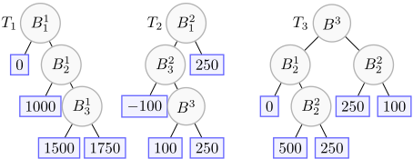
A term t over B = {B1, . . . ,Bp} is a conjunctivelyinterpreted set of literals over B. ⊤ denotes the term associated with the empty set of literals. t is canonical when it contains one literal per Boolean condition in B. Such a term thus corresponds to a truth assignment over B. Every instance x ∈ X can be associated with a canonical term tx over B such that for every i ∈ [p], Bi (resp. ¬Bi) belongs to tx if and only if x satisfies (resp. does not satisfy) the condition Bi. A term t over B covers an instance x ∈ X whenever t ⊆ tx. Deciding whether t covers x can be achieved in time linear in |t| and |x|.
Every term t over B that is consistent (i.e., t does not contain both an element of B and its negation) can be simplified using Σ. Thus, each time t contains two distinct literals ℓ and ℓ′ such that ℓ′ is entailed by ℓ given Σ, ℓ′ can be removed from t. The specific nature of Σ ensures that such a simplification process is confluent, i.e., the term obtained at the end of the simplification process (called the simplification of t given Σ) is uniquely defined whatever the ordering according to which the literals are considered (this would not be ensured if Σ was any formula over B). Thus, when simplified, t cannot contain more than one positive (resp. negative) literal issued from the same numerical attribute Ai and more than one positive literal issued from the same categorical attribute Ai (and if such a positive literal exists, t does not contain any negative literal issued from Ai). By construction, the simplification of t given Σ is equivalent to t under Σ. Furthermore, the simplification of t given Σ can be computed in time O(|Σ| · |t|2 ).
3 On Abductive Explanations for Boosted Regression Trees
Let F be a boosted tree over A. Suppose that t is a term over B that covers x ∈ X. In the classification case, t is viewed as an abductive explanation for x given F when every instance x′ covered by t is classified as x by F : F (x′ ) = F (x). Thus, any t is (or is not) an abductive explanation for x given F depending on the evaluation of this condition. In the regression case, every t is more or less an abductive explanation for x given F, i.e., the F-value of every instance x′ covered by t is more or less distant to F(x). Accordingly, a notion of imprecision of t can be defined.
Definition 1. Let F be a boosted regression tree over A and t a term over B. The imprecision of t is defined as the length Lt = Mt -mt of the interval It = [mt,Mt] induced by t and defined by mt = min({F (x) : x ∈ X, t covers x}) and Mt = max ({F (x) : x ∈ X, t covers x}).
A monotonic relationship exists between the generality of the terms t over B that can serve as abductive explanations and the lengths of the corresponding intervals It:
Proposition 1. Let F be a boosted regression tree over A, and t, t′ two terms over B. If t ⊆ t′ holds then It ⊇ It′ holds, so that Lt ≥ Lt′ .
Generating abductive explanations We are interested in explaining the values predicted by boosted regression trees using abductive explanations defined as follows:
Definition 2. Let F be a boosted regression tree over A, x ∈ X an instance, and I an interval over the reals. A term t over B is
- an abductive explanation for x given F and I if and only if t covers x and for every instance x′ ∈ X that is covered by t, we have F(x′ ) ∈ I.
- a subset-minimal abductive explanation for x given F and I if and only if t is an abductive explanation for x given F and I and no proper subset of t is an abductive explanation for x given F and I.
Among the abductive explanations for x is its direct reason tFx , defined as the union over the trees Ti ∈ F of the sets of literals (one per tree Ti) containing the literals encountered in the unique path of Ti that is compatible with tx. By construction, tFx ⊆ tx is an abductive explanation for x given F and any I containing F(x). As every abductive explanation for x given F and I (whatever I), tFx is consistent with Σ (otherwise, it would not cover x). However, tFx can be highly redundant (i.e., in general, it is not a subset-minimal abductive explanation for x given F and I).
A standard approach to the generation of a subset-minimal abductive explanation consists of taking advantage of a greedy algorithm. Our greedy algorithm G to compute a subset-minimal abductive explanation for x given F and I considers at start the canonical term tx over B (actually, any term t over B that covers x can do the job, thus we could start with tFx or its simplification instead). G proceeds as follows. It tries to eliminate successively literals ℓ from t. Thus, each time t \{ℓ} still satisfies the coverage condition induced by I, ℓ is removed from t, otherwise it is kept. Accordingly, implementing this approach mainly amounts to deciding the coverage condition. However, this is a computationally hard problem:
Proposition 2. Let F be a boosted regression tree over A, x ∈ X an instance, and I an interval over the reals. Let t be a term over B. Deciding whether t is an abductive explanation for x given F and I is coNP-complete.
Therefore, G uses first an incomplete, yet polynomial-time approximate coverage test, using a method close to the one used for generating (subset-minimal) abductive explanations given a boosted classification tree, as described in [Audemard et al., 2023]. When the approximate coverage test succeeds, ℓ can be removed from t for sure. When the test fails, ℓ is kept even but this does not imply that t \ {ℓ} necessarily violates the exact coverage test. What makes those approximate coverage tests appealing is that they can be achieved very efficiently and that, empirically, they often lead to the removal of many literals from the term t one started with. Then, a second pass of G over the remaining literals, using this time expensive, but exact, coverage tests, ensure that the resulting term is a subset-minimal abductive explanation for x given F and I. Each exact coverage test is achieved using a constraintbased encoding of the coverage condition and the use of a solver on the encoding. Each of the two passes takes account for the constraint Σ about the attributes from B so that any truth assignment over B that violates Σ is discarded, as in [Gorji and Rubin, 2022]. Notably, G exhibits an anytime behaviour. At each step after the initialization, the current term t provably is an abductive explanation for x given F and I. When more time is allocated to the algorithm, the generality of t may only increase and if the algorithm is not interrupted, a subset-minimal abductive explanation for x given F and I is returned. Furthermore, it is guaranteed that the subsetminimal abductive explanation produced by G whenever it terminates normally is simplified.
A constraint-basedmodel for the exact coverage test Let us now explain how to build a constraint-based model Mg that can be used to achieve an exact coverage test, i.e., to decide whether a given term t is an abductive explanation for x given F and I. Mg contains MILP constraints and indicator constraints (which are supported by the solver used, namely CPLEX [Cplex, 2009]). We start by defining a set of MILP constraints over B encoding the corresponding domain theory Σ:
t is represented by the following MILP constraints:
Each tree Ti of F is represented by its set of terms {ti1 , . . . , tipi }, where each term gathers the literals representing the conditions that are true in a root-to-leaf path of Ti. Each tij (j ∈ [pi]) characterizes a unique path of Ti and wij is the real number labelling the leaf of the j th path. With each tree Ti (i ∈ [m]) we associate a set of Boolean variables Li = {Liti1 , . . . , Litipi }, such that Litij (j ∈ [pi]) is true when the conditions given by tij are met. For all i ∈ [m], the following set of MILP constraints indicates how each Litij is connected to the Boolean variables of B:
Because Ti is a decision tree, the terms in {ti1 , . . . , tipi } are orthogonal (i.e., pairwise inconsistent). This implies that exactly one Litij must be set to true, which is ensured by the following set of MILP constraints:
We also consider a set of continuous variables W = {W1, . . . , Wm} and some constraints that associate with each tree Ti (i ∈ [m]) the real number Wi that corresponds to the value of Ti for a selected root-to-leaf path made precise by a truth assignment over Li. Each Wi (i ∈ [m]) is defined by the following MILP constraints:
Let FW be a continuous variable that represents the value of the regression tree for any truth assignment over B. The following linear constraint computes FW:
Given a non-empty interval I = (lb, ub), a term t over B is an abductive explanation for x given F and I when it is impossible to find a truth assignment over B that extends t and such that such that (FW ≤ lb) or (FW ≥ ub) holds. This disjunction is represented using the following constraints, involving two binary variables IL and IU which serve as indicator variables:
By construction, t is an abductive explanation for x given F and I if and only if the model Mg gathering all the constraints above is inconsistent. Note that when I = ∅, no computation is required since no abductive explanation for x given F and I may exist. Finally, when I is a singleton (e.g., I = {F (x)}), we can use (F (x) - ϵ, F (x) + ϵ) as the initial interval, where ϵ > 0 is a preset threshold that is as small as expected.
Example 3. Consider I1 = [1750, 2250] and I2 = [1500, 2500], which contain the F-value (2000) of xex = (2200$, "self-employed", 1).
xex has two subset-minimal abductive explanations given F and I1: {B1 2 , B2 3 ,B3 } and {B1 2 , B1 3 , B2 3 }. This means that to get an amount of loan granted between 1750$ and 2250$ the applicant's incomes must exceed 2000$, he/she has to be self-employed and married, or the applicant's incomes must exceed 2000$ but not exceed 3000$ and he/she has to be selfemployed.
xex has a unique subset-minimal abductive explanation given F and I2: {B1 2 }. This means that to get an amount of loan granted between 1500$ and 2500$ the applicant's incomes must exceed 2000$.
Evaluating abductive explanations Once an abductive explanation t for x given F and an interval I has been computed (or a candidate t covering x and consistent with Σ is pointed out by the human user who wants to get some explanations - aka the explainee [Miller, 2019]), it is interesting to be able to evaluate its imprecision. Indeed, it can be the case that I ̸= It. To be more specific, if t is an abductive explanation t for x given F and I, then only It ⊆ I is ensured. Computing It and its length is thus a valuable approach to determine to which extent the actual imprecision Lt of the explanation t differs from the admissible imprecision considered initially by the explainee (the length of I). However, identifying It is computationally demanding in general, as a consequence of the following proposition, which is close to Proposition 2 but considers different inputs (no instance x is considered as an input in Proposition 3).
Proposition 3. Let F be a boosted regression tree over A, and I an interval over the reals. Let t be a term over B such that t ∧Σ is consistent. Deciding whether every instance x ∈ X covered by t is such that F(x) ∈ I is coNP-complete.
In our algorithm E, the problem of deriving It is tackled using binary search (finding the two bounds mt, Mt of It). At each step, in order to determine whether a given value is an admissible lower bound of mt (or an upper bound of Mt), a constraint-based encoding of the condition is produced and a solver is used to address the corresponding decision problem. To ensure the termination of the search, a preset threshold ϵ is used when the distance between the two successive values that have been computed is lower than ϵ. By construction, E also has an anytime behaviour: if E is stopped then the interval I given by the current lower (resp. upper) bound of mt (resp. Mt) is such that It ⊆ I. I can then be viewed as an upper approximation of It.
A constraint-based model for finding bounds for It Let us explain how to determine mt or a lower bound of it (identifying Mt or an upper bound of it is similar). Let Me be the constraint-based model containing every constraint from Mg, but Equation (9). We consider two variables lower and lowerb such that at each step of the binary search, mt provably belongs to [lowerb, lower]. At start, lowerb is set to mF = ∑ni=1 min(Ti) and lower is set to F(xt) where xt is any instance over B that satisfies t ∧ Σ. Note that xt can be computed in linear time from t and Σ because t ∧ Σ is a 2-CNF formula [Even et al., 1976]. Let mid = lower+lowerb 2 . If Me ∧(FW ≤ mid) is inconsistent, then mid is an acceptable lower bound of mt, so that lowerb can be set to mid. In the remaining case when Me ∧ (FW ≤ mid) is consistent, instead of setting lower to mid, lower can be safely set to FW, since FW is an upper bound of mt that is at least as good as mid given that FW ≤ mid holds. Then, the binary search resumes using the updated bounds. Clearly, using FW instead of mid in the case when Me ∧ (FW ≤ mid) is consistent leads to boost the binary search.
Example 4. Here are some terms t over B covering the instance xex considered in the running example and the corresponding least intervals It.
t3 and t5 are the subset-minimal abductive explanations for xex given F and I = [1750, 2250]. We have both It3 ⊂ I and It5 ⊂ I.
4 Empirical Evaluation
The generation algorithm G and the evaluation algorithm E have been assessed on several datasets in order to figure out the extent to which they are practical.
Experimental setup The empirical protocol we considered was as follows. We have focused on 10 datasets for regression, which are standard benchmarks found on the web sites kaggle (https://www.kaggle.com/), UC Irvine Machine Learning Repository (https://archive.ics.uci.edu/ml/ index.php) or openML (https://www.openml.org/). These datasets are described in Table 1.
For each dataset, the algorithms XGBoost [Chen and Guestrin, 2016] and LightGBM [Ke et al., 2017] have been used to learn boosted regression trees. Numerical attributes have been binarized on-the-fly by the boosted tree learning algorithms. Categorical attributes have been one-hot encoded. All the hyper-parameters of the two learning algorithms have been set to their default values (100 trees per forest, with a depth at most 6 for XGBoost and a number of leaves at most 31 for LightGBM). Thus, no tuning has been performed. Indeed, our purpose is to evaluate the performance of G and E, whatever the quality of the boosted regression trees we started with. Hence, our experiments have concerned both accurate predictors, and predictors exhibiting rather low accuracies. For each dataset, each boosted tree has been learned from a training set containing 80% of the dataset, and its accuracy was measured as its mean R2 score [Ling and Kenny, 1981] over the remaining 20% of the dataset.
| Name | #A | #N | #C | #B | #I |
|---|---|---|---|---|---|
| Winequality-red | 11 | 0 | 0 | 11 | 1599 |
| Winequality-white | 11 | 0 | 0 | 11 | 4898 |
| CreditcardFraudDet. | 29 | 0 | 0 | 29 | 284807 |
| l4d2-player-stats-final | 112 | 111 | 1 | 0 | 20830 |
| Houses-prices | 46 | 26 | 20 | 0 | 2919 |
| Steel ind. energy cons. | 9 | 6 | 3 | 0 | 35040 |
| Bike sharing: hour | 15 | 13 | 0 | 2 | 17379 |
| Bike sharing: daily | 13 | 11 | 0 | 2 | 731 |
| NASA airfoil self-noise | 5 | 5 | 0 | 0 | 1503 |
| abalone | 9 | 8 | 1 | 0 | 4177 |
| Dataset / Boosted Tree | Instance / Direct Reason | I 0.5 F,x | I 2.5 F,x | |||||||||||
|---|---|---|---|---|---|---|---|---|---|---|---|---|---|---|
| Name | R2 #Cond | SizeI | SizeD | SizeG | TOG | TimeG | %Red | TOE TimeE | SizeG | TOG | TimeG | %Red | TOE TimeE | |
| Winequality-red | 0.42 | 666 | 21.5(±0.8) | 21.4(±0.9) | 21.2(±1.2) | 0 | 2.2(±0.3) | 20.9(±23.2) | 0 | 0.8(±0.0) 19.9(±1.5) | 0 | 2.5(±0.3) | 18.6(±12.1) | 0 0.9(±0.1) |
| Winequality-white | 0.46 | 764 | 21.8(±0.6) | 21.8(±0.6) | 21.4(±0.8) | 0 | 2.2(±0.2) | 20.2(±16.8) | 0 0.8(±0.0) | 19.9(±1.2) | 0 | 2.5(±0.3) | 18.1(±12.1) | 0 0.9(±0.1) |
| CreditcardFraudDet. | 0.96 | 1506 | 56.0(±1.8) | 39.9(±2.0) | 25.7(±3.9) | 4 | 216(±244) | 8.9(±6.0) | 22 258(±301) | 18.8(±2.4) | 90 | 770(±207) | 25.1(±11.8) | 97 806(±97.6) |
| l4d2-player-stats-final | -2.62 | 1378 | 171(±18.9) | 95.4(±10.9) | 56.2(±7.1) | 98 | 4.8(±0.3) | 18.1(±7.6) | 96 172(±175) | 15.6(±2.6) | 100 | - | 52.2(±7.9) | 100 - |
| Houses-prices | 0.88 | 897 | 61.8(±6.8) | 62.2(±8.0) | 49.5(±8.6) | 0 | 5.9(±1.0) | 5.6(±4.7) | 0 2.2(±0.7) | 33.9(±10.1) | 0 | 72.2(±132) | 2.6(±2.3) | 0 52.0(±98.3) |
| Steel ind. energy cons. | 0.99 | 533 | 13.5(±2.4) | 11.2(±1.5) | 7.0(±2.0) | 0 | 1.5(±0.2) | 36.8(±15.7) | 0 1.0(±0.2) | 5.0(±1.5) | 0 | 1.6(±0.3) | 44.6(±17.7) | 0 1.9(±0.5) |
| Bike sharing: hour | 0.99 | 603 | 20.0(±2.0) | 11.2(±2.1) | 3.7(±0.7) | 0 | 1.5(±0.3) | 42.6(±19.2) | 0 1.4(±0.2) | 3.2(±0.7) | 0 | 1.4(±0.2) | 33.0(±13.1) | 0 2.0(±0.3) |
| Bike sharing: daily | 0.99 | 618 | 19.3(±1.2) | 18.1(±1.4) | 10.9(±1.6) | 0 | 1.8(±0.5) | 16.9(±9.1) | 0 1.5(±0.8) | 4.0(±0.8) | 0 | 4.0(±3.5) | 30.7(±10.6) | 0 61.9(±65.1) |
| NASA airfoil self-noise | 0.92 | 149 | 8.8(±0.8) | 8.8(±0.8) | 8.5(±1.0) | 0 | 1.2(±0.3) | 68.5(±21.0) | 0 0.8(±0.0) | 7.3(±1.1) | 0 | 1.2(±0.3) | 48.1(±18.8) | 0 1.0(±0.2) |
| abalone | 0.99 | 456 | 17.0(±0.3) | 16.8(±0.7) | 2.1(±0.6) | 0 | 1.6(±0.4) | 90.1(±8.3) | 0 0.9(±0.0) | 2.0(±0.1) | 0 | 1.5(±0.5) | 97.5(±8.1) | 0 1.1(±0.2) |
In order to evaluate G, we needed to consider intervals I. To this purpose, for each dataset and each boosted tree F , we have first estimated the range of values that can be reached by F = {T1, . . . , Tm}. This estimate is given by the interval IF = [mF ,MF ] where MF = ∑ni=1 max(Ti) echoes mF = ∑ni=1 min(Ti). IF can be computed in time linear in |F|. Note that while the image F(X) and its superset given by the interval I⊤ are guaranteed to be included in IF , 1 interval IF does not coincide with I⊤ in general 2 (the minimal or maximal leaves over the trees of F may easily correspond to incompatible paths). The length LF = MF -mF of IF gave us a range of values that can be used to define intervals I of various lengths containing F(x) (whatever x) and reflecting various imprecision levels about the F-predicted value of x. Thus, for any x ∈ X and any r ∈ [0, 100], we defined
Centered intervals I rF,x have been considered for the ease of empirical protocol, only. 3 Indeed, our algorithm G can take any interval I as input, provided that F(x) ∈ I. Then, for each dataset, each boosted tree F and a pool of 100 instances x ∈ X drawn uniformly at random from the test set, we have computed the simplification of the direct reason tFx and we have run G in order to derive a subset-minimal abductive explanation t for x given F and I rF,x where r ∈ {0.5, 1, 2.5, 5, 10}. We took advantage of the CPLEX solver [Cplex, 2009] in this computation.
Finally, in order to assess the performance of E, we started from the subset-minimal abductive explanations t for x given F and I rF,x (where r ∈ {0.5, 1, 2.5, 5, 10}) that have been computed by G, and derived from them using the evaluation algorithm the corresponding intervals It and we measured their lengths. Using the terms t computed by G in our experiments was a natural choice, but other alternatives were possible (the two algorithms E and G are completely independent and they can be used separately). The parameter ϵ used in E has been set to 0.01 in our experiments.
1 Let us recall that ⊤ denotes the empty conjunction of literals.
2 Note that, unlike what happens in the general case, we have IF = I⊤ for the running example.
3 Instead of I rF,x, we could have considered intervals generated from prediction interval estimators (see Section 5).
For each dataset, each boosted tree F , we counted the number of instances x ∈ X (out of 100) for which a subsetminimal abductive explanation has been computed in due time given F and each of the 5 intervals I rF,x that have been considered (a time-out (TO) of 900s has been considered per instance and interval). For each instance for which the computation has been successful, we measured the time needed to get the result and the size of the resulting subset-minimal abductive explanation t. Then we counted the number of resulting terms t for which the evaluation algorithm terminates in due time (using a TO of 600s for each bound). We measured the time required to derive It, and the length Lt of this interval in order to compare it with the length 2r 100 · LF of the interval I rF,x that has been considered when computing t. Especially, we measured the reduction of the imprecision that is obtained. This reduction is defined by 0 when LF = 0 and by 2r 100 ·LF -Lt 2r 100 ·LF in the remaining case. All the experiments have been conducted on a computer equipped with Intel(R) XEON E5-2637 CPU @ 3.5 GHz and 128 Gib of memory.
Experimental results Table 2 presents some empirical results obtained for the ten datasets that have been considered. The leftmost column of Table 2 gives the name of the dataset b. Columns R2, #Cond, SizeI and SizeD give, respectively, the R2 score of the boosted tree F learned using LightGBM, the number of distinct Boolean conditions occurring in it, the mean and standard deviation of the lengths of the simplified instances over B, and finally, the mean and standard deviation of the lengths of the associated simplified direct reasons. Then, for each interval I rF,x considered (r = 0.5 and r = 2.5 in Table 2), we report the mean and standard deviation of the sizes of the abductive explanations t (that have been computed using G), and the mean and standard deviation of the reductions of the interval considered for deriving t (the reductions are computed using E), the number of timeouts and the mean time and standard deviation of the computation times (in seconds) when the corresponding algorithm (G or E) terminated in due time. 4
In light of the experiments, G and E appear as practical for boosted trees involving a significant number of Boolean conditions (up to 800). This corresponds to the boosted trees computed using LightGBM on every dataset but the larger ones, namely l4d2-player-stats-final, creditCardFraudDetection, and houses-prices. Thus, for the seven other datasets, no timeout has occurred during the computations and the mean computation times for deriving a subset-minimal abductive explanation for any of the instance (out of 100) never exceeded 90 seconds (and most of the time, only a couple of seconds was required). A valuable observation is that both G and E provide useful outputs even when they are interrupted before a normal termination.
4 For space reasons, more detailed results including results about the boosted trees learned using XGBoost and/or concerning other values of r are not reported here, but they can be found in the supplementary material.
In practice, the sizes of the explanations generated using G can be much smaller than the sizes of the instances they explain, and much smaller than the sizes of the corresponding direct reasons. For instance, considering the line associated with the dataset bike sharing: daily and the columns SizeI, SizeD and SizeG (for r = 0.5) in Table 2, we can check that the subset-minimal abductive explanations that have been computed are of average size 3.7, while the corresponding instances are of average size 20 and their direct reasons are of average size 11.2. Table 2 also shows that the the reduction of the imprecision that is achieved by E is significant most of the time.
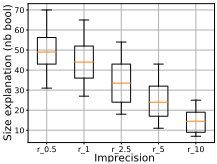
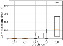
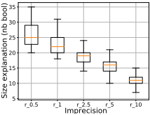
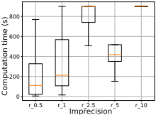
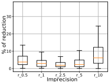
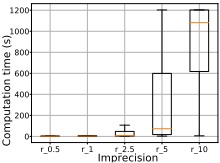
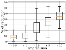
Our experiments have also permitted to assess on a qualitative, yet empirical basis the connections between the generality of the explanations (given by their sizes) and the imprecision considered at start for generating them using G. We illustrate them on two datasets: houses-prices and creditcard. Figure 2 (left) (resp. Figure 3 (left)) gives box plots synthesizing the distribution of sizes of the subset-minimal abductive explanations that have been generated for various values of r for the boosted tree trained on houses-prices (resp. creditcard) using LightGBM. Figure 2 (right) (resp. Figure 3 (right)) is about the corresponding computation times. Figure 4 and Figure 5 report similar results about the reductions of the intervals considered as input by G (left) and the corresponding computation times (right).
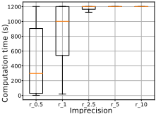
We can observe on Figure 2 (left) that the sizes of the explanations significantly decrease when the admissible imprecision increases. Contrariwise, the computation times (see Figure 2 (right)) increase when the admissible imprecision increases (more literals must be removed by the greedy generation algorithm to get subset-minimal abductive explanations).
Figure 4 (left) and Figure 5 (left) show that the reduction of the imprecision that is achieved by E can be important, and Figure 4 (right) and Figure 5 (right) show that the computation times typically increase when the generality of the term considered at start increases (this can be easily explained by the fact that the number of instances covered by the term increases as well). For each of G and E, we observed that the standard deviation of the computation times is sometimes high (larger than the mean). Similar observations can be done for the other datasets. 5
5 Other RelatedWork
Most existing work about XAI for regression exploits solutions developed for the classification task, reducing regression into (multi-class) classification. This is typically achieved through a partitioning of the reals into intervals, requiring the elicitation of decision boundaries that can be more or less arbitrary. Once done, popular XAI techniques for classification can be leveraged. Thus, [Strumbelj and Kononenko, 2011] presents an approach to explanation based on the notion of feature importance. [Kontokosta, 2019;
5 Additional box plots are provided in the supplementary material.
Moore and Bell, 2022] use Shapley values and take advantage of them in the context of two applications (energy efficiency of buildings and prediction of myocardial infarction). What makes such XAI approaches appealing is that they are model-agnostic and scalable, so they can be used to explain predictions achieved by very powerful ML models (e.g., deep neural nets). The (heavy) price to be paid is that they do not offer any formal insurance of rigor [Ignatiev, 2020].
Contrariwise, our approach to XAI is specific to boosted regression trees. However, the (subset-minimal) abductive explanations that are generated by G and evaluated by E are provably correct. This correctness guarantee comes from the logical setting considered for representing boosted trees and the use of automated reasoning tools for deriving (and evaluating) explanations. This makes our work relevant to formal XAI [Marques-Silva and Ignatiev, 2022].
Prior work in formal XAI that have been concerned with tree ensembles have mainly focused on the computation of contrastive explanations (see, for instance, [Cui et al., 2015; Kanamori et al., 2020; Parmentier and Vidal, 2021; Hada and Carreira-Perpi˜n´an, 2021]) and on the classification issue (see, for instance, [Choi et al., 2020; Izza and MarquesSilva, 2021; Audemard et al., 2022; Ignatiev et al., 2019b; 2022]). Thus, they are significantly different from our own work, centered on abductive explanations for regression.
Estimating prediction intervals is a well-established topic in Machine Learning (or even in traditional statistics), and is widely used in practice. A number of approaches for estimating prediction intervals have been pointed out so far (e.g., via quantile regression [Koenker, 2005]) and they are based a variety of techniques (e.g., the jacknife method [Barber et al., 2021]). The main goal is to measure the robustness of the predictor and to control the use of the predictor by exploiting statistical guarantees. Accordingly, those approaches are focused on instances, not on explanations for instances, while our algorithm E is about the evaluation of abductive explanations, with logic-based guarantees, which is quite a different perspective. Note nevertheless that the output of prediction interval estimators could be used to define intervals used as inputs by our algorithm G.
Finally, [Letzgus et al., 2022] identifies important conditions about the regression problem that should be considered when developing dedicated XAI approaches, but are not always guaranteed by XAI approaches to classification. One of them states that explanations should be produced relative to some reference value. Our algorithm G takes such a reference value into account, represented by an interval I. As we have shown both in theory and in practice, the choice of I may substantially affect the subset-minimal abductive explanations that are derived.
6 Conclusion
We have presented and assessed two anytime algorithms G and E for generating (resp. evaluating) abductive explanations for boosted regression trees. The datasets used for learning the boosted trees can be based on data of mixed type (including categorical and numerical attributes). This leads to boosted trees containing Boolean conditions that are not independent in general. In our approach, the underlying domain theory is used to ensure that the abductive explanations that are generated are not unnecessarily specific, but also to simplify the explanations. Most of the time, our algorithms can be used to generate (resp. evaluate) in a few seconds abductive explanations for boosted regression trees based on a large number of Boolean conditions (up to 800). A valuable observation is that, in general, the (subset-minimal) abductive explanations that are generated using G are significantly smaller than the initial descriptions of the instances in terms of Boolean attributes. Furthermore, the reduction of the imprecision that is achieved by E can be very significant as well.
Notably, the correctness of G (resp. E) does not require any specific assumption on the way the ensemble of regression trees F used as input has been learned. Thus, G and E are applicable to general regression forests, and not only to boosted regression trees, and provide the same guarantees for general regression forests as the ones offered for boosted regression trees. Especially, it does not matter if bagging has been used instead of boosting as an ensemble learning method, so that F actually is a random forest. Note nevertheless that for random forests, the computation of a prediction interval that could be used as an input of G is much easier than for boosted trees, since trees in a random forest are independently generated.
As illustrated by our experiments, it can be the case that the size of the explanations produced by G is quite large. In such a case, pieces of knowledge (when available) can be leveraged to try to simplify the explanations further. However, it may happen that simplified explanations are still too large to be viewed as intelligible enough by the explainee. It is important to keep in mind that such a situation does not reflect a drawback of the XAI approach (which aims at explaining the behaviour of the predictor as it is, and not as it could be), but a feature of the predictor itself. Indeed, the fact that the explanations are large indicates that many attributes are needed to explain the regression value that has been computed. Knowing it, the explainee is free to decide what to do with the value and the predictor (trust in it or not).
This work calls for a number of perspectives. One of them is to focus on a specific application where the expertise of a human user can be exploited to assess the quality of the explanations that are generated. We are confident that the possibility of computing It given t and F can be leveraged to design interaction protocols with an explainee, in the objective of providing explanations that achieve a good generality/precision trade-off and fitting the expectations of the explainee [Doshi-Velez and Kim, 2017; Narayanan et al., 2018]. An example of such a process (with the explainee-in-the-loop) would be as follows: starting from x and an interval I furnished by the explainee, one first computes a subset-minimal explanation t for x and I using G and then evaluates it using E by computing It. If the explainee finds t too specific, then one asks her/him for a subset of literals t′ to be removed from t in order to make t more general and evaluate the term t\t′ . If the precision Lt\t′ is fine with the explainee, we can stop the interaction and return t \ t′ . If it is deemed too large, one can resume at the first step and look for another subset-minimal explanation for x and I.
Acknowledgments
Many thanks to the anonymous reviewers for their comments and insights. This work has benefited from the support of the AI Chair EXPEKCTATION (ANR-19-CHIA-0005-01) of the French National Research Agency. It was also partially supported by TAILOR, a project funded by EU Horizon 2020 research and innovation programme under GA No 952215.
@inproceedings{ijcai2023p382,
  title     = {Computing Abductive Explanations for Boosted Regression Trees},
  author    = {Audemard, Gilles and Bellart, Steve and Lagniez, Jean-Marie and Marquis, Pierre},
  booktitle = {Proceedings of the Thirty-Second International Joint Conference on
               Artificial Intelligence, {IJCAI-23}},
  publisher = {International Joint Conferences on Artificial Intelligence Organization},
  editor    = {Edith Elkind},
  pages     = {3432--3441},
  year      = {2023},
  month     = {8},
  note      = {Main Track},
  doi       = {10.24963/ijcai.2023/382},
  url       = {https://doi.org/10.24963/ijcai.2023/382},
}
TY - CPAPER TI - Computing Abductive Explanations for Boosted Regression Trees AU - Audemard, Gilles AU - Bellart, Steve AU - Lagniez, Jean-Marie AU - Marquis, Pierre T2 - Proceedings of the Thirty-Second International Joint Conference on Artificial Intelligence, IJCAI-23 PB - International Joint Conferences on Artificial Intelligence Organization PY - 2023 SP - 3432 EP - 3441 DO - 10.24963/ijcai.2023/382 UR - https://doi.org/10.24963/ijcai.2023/382 ER -Copied
Machine-readable versions of this paper, for tools and AI agents:





