
ReLiNet: Stable and Explainable Multistep Prediction with Recurrent Linear Parameter Varying Networks
Proceedings of the Thirty-Second International Joint Conference on Artificial Intelligence. Main Track. Pages 3461-3469.
https://doi.org/10.24963/ijcai.2023/385
Keywords
- AI Ethics, Trust, Fairness: ETF: Explainability and interpretability
- AI Ethics, Trust, Fairness: ETF: Safety and robustness
- Machine Learning: ML: Recurrent networks
Abstract
Multistep prediction models are essential for the simulation and model-predictive control of dynamical systems. Verifying the safety of such models is a multi-faceted problem requiring both system-theoretic guarantees as well as establishing trust with human users. In this work, we propose a novel approach, ReLiNet (Recurrent Linear Parameter Varying Network), to ensure safety for multistep prediction of dynamical systems. Our approach simplifies a recurrent neural network to a switched linear system that is constrained to guarantee exponential stability, which acts as a surrogate for safety from a system-theoretic perspective. Furthermore, ReLiNet's computation can be reduced to a single linear model for each time step, resulting in predictions that are explainable by definition, thereby establishing trust from a human-centric perspective. Our quantitative experiments show that ReLiNet achieves prediction accuracy comparable to that of state-of-the-art recurrent neural networks, while achieving more faithful and robust explanations compared to the model-agnostic explanation method of LIME.
- [Alvarez Melis and Jaakkola, 2018] David Alvarez Melis and Tommi Jaakkola. Towards robust interpretability with self-explaining neural networks. In NeurIPS, volume 31.
- Curran Associates, Inc., 2018.
- [Baier and Frank, 2023] Alexandra Baier and Daniel Frank. deepsysid: System Identification Toolkit for Multistep Prediction using Deep Learning. https://doi.org/10.18419/ darus-3455, 2023. Accessed: 2023-05-24. DOI
- [Baier and Staab, 2022] Alexandra Baier and Steffen Staab. A Simulated 4-DOF Ship Motion Dataset for System Iden- tification under Environmental Disturbances. https://doi. org/10.18419/darus-2905, 2022. Accessed: 2023-05-24. DOI
- [Baier et al., 2023] Alexandra Baier, Decky Aspandi, and Steffen Staab. Supplements for "ReLiNet: Stable and Explainable Multistep Prediction with Recurrent Linear Parameter Varying Networks". https://doi.org/10.18419/ darus-3457, 2023. Accessed: 2023-05-24. DOI
- [Bamieh and Giarré, 2002] Bassam Bamieh and Laura Gi- arré. Identification of linear parameter varying models. Int. J. Robust and Nonlinear Control, 12(9):841-853, 2002.
- [Bhatt et al., 2020] Umang Bhatt, Adrian Weller, and José M. F. Moura. Evaluating and aggregating feature-based model explanations. In IJCAI, pages 3016-3022, 7 2020. IJCAI
- [Bohle et al., 2021] Moritz Bohle, Mario Fritz, and Bernt Schiele. Convolutional dynamic alignment networks for interpretable classifications. In CVPR, pages 10029- 10038, June 2021.
- [Böhle et al., 2022] Moritz Böhle, Mario Fritz, and Bernt Schiele. B-cos networks: Alignment is all we need for interpretability. In CVPR, pages 10329-10338, June 2022.
- [Bonassi et al., 2021] Fabio Bonassi, Marcello Farina, and Riccardo Scattolini. On the stability properties of gated recurrent units neural networks. Systems & Control Let- ters, 157:105049, 2021.
- [Brendel and Bethge, 2019] Wieland Brendel and Matthias Bethge. Approximating CNNs with bag-of-local-features models works surprisingly well on imagenet. In ICLR, 2019.
- [Chattopadhyay et al., 2022] Aditya Chattopadhyay, Stewart Slocum, Benjamin D. Haeffele, Rene Vidal, and Donald Geman. Interpretable by design: Learning predictors by composing interpretable queries, 2022. https://arxiv.org/ abs/2207.00938. Link
- [Chen et al., 2017] Shaofeng Chen, Yang Cao, Yu Kang, Rongrong Zhu, and Pengfei Li. Deep CNN Identifier for Dynamic Modelling of Unmanned Helicopter. In NeurIPS, pages 51-60, Cham, 2017.
- [Chen et al., 2019] Chaofan Chen, Oscar Li, Daniel Tao, Alina Barnett, Cynthia Rudin, and Jonathan K Su. This looks like that: Deep learning for interpretable image recognition. In NeurIPS, volume 32.
- Curran Associates, Inc., 2019.
- [Du et al., 2020] Yingwei Du, Fangzhou Liu, Jianbin Qiu, and Martin Buss. A semi-supervised learning approach for identification of piecewise affine systems. IEEE Trans. on Circuits and Systems I, 67(10):3521-3532, 2020.
- [Genc, 2017] Sahika Genc. Parametric system identifica- tion using deep convolutional neural networks. In IJCNN, pages 2112-2119, 2017.
- [Guidotti and Ruggieri, 2019] Riccardo Guidotti and Salva- tore Ruggieri. On the stability of interpretable models. In IJCNN, pages 1-8, 2019.
- [Hojjatinia et al., 2020] Sarah Hojjatinia, Constantino M. Lagoa, and Fabrizio Dabbene. Identification of switched autoregressive exogenous systems from large noisy datasets. Int. J. Robust and Nonlinear Control, 30(15):5777-5801, 2020.
- [Jinil and Reka, 2019] Nectar Jinil and Sofana Reka. Deep learning method to predict electric vehicle power require- ments and optimizing power distribution. In ICEES, pages 1-5, 2019.
- [Krishnapriyan et al., 2021] Aditi Krishnapriyan, Amir Gholami, Shandian Zhe, Robert Kirby, and Michael W. Mahoney. Characterizing possible failure modes in physics-informed neural networks. In NeurIPS, 2021.
- [Lauer, 2013] Fabien Lauer. Estimating the probability of success of a simple algorithm for switched linear regres- sion. Nonlinear Analysis: Hybrid Systems, 8:31-47, 2013.
- [Lauer, 2015] Fabien Lauer. On the complexity of piecewise affine system identification. Automatica, 62(C):148-153, 2015.
- [Letzgus et al., 2022] Simon Letzgus, Patrick Wagner, Jonas Lederer, Wojciech Samek, Klaus-Robert Müller, and Grégoire Montavon. Toward Explainable Artificial In- telligence for Regression Models: A methodological per- spective. IEEE Signal Processing Magazine, 39(4):40-58, 2022.
- [Li et al., 2017] Guoyuan Li, Bikram Kawan, Hao Wang, and Houxiang Zhang. Neural-network-based modelling and analysis for time series prediction of ship motion. Ship Technology Research, 64, 2017.
- [Li et al., 2019] Kai Li, Jiaqing Kou, and Weiwei Zhang. Deep neural network for unsteady aerodynamic and aeroe- lastic modeling across multiple mach numbers. Nonlinear Dynamics, 96:1-21, 2019.
- [Lin and Antsaklis, 2009] Hai Lin and Panos J. Antsaklis. Stability and stabilizability of switched linear systems: A survey of recent results. IEEE Trans. Automatic Control, 54(2):308-322, 2009.
- [Lundberg and Lee, 2017] Scott M Lundberg and Su-In Lee. A unified approach to interpreting model predictions. In NeurIPS, volume 30.
- Curran Associates, Inc., 2017.
- [Ma and Qu, 2020] Lijing Ma and Shiru Qu. A se- quence to sequence learning based car-following model for multi-step predictions considering reaction delay. Transportation Research Part C: Emerging Technologies, 120:102785, 2020.
- [Marcos et al., 2020] Diego Marcos, Ruth Fong, Sylvain Lo- bry, Remi Flamary, Nicolas Courty, and Devis Tuia. Con- textual semantic interpretability. In ACCV, November 2020.
- [Massucci et al., 2021] Louis Massucci, Fabien Lauer, and Marion Gilson. Regularized switched system iden- tification: a statistical learning perspective. IFAC- PapersOnLine, 54(5):55-60, 2021. 7th IFAC Conference on Analysis and Design of Hybrid Systems ADHS 2021.
- [Mayne et al., 2000] D.Q. Mayne, J.B. Rawlings, C.V. Rao, and P.O.M. Scokaert. Constrained model predictive con- trol: Stability and optimality. Automatica, 36(6):789-814, 2000.
- [Mejari et al., 2020] Manas Mejari, Vihangkumar V. Naik, Dario Piga, and Alberto Bemporad. Identification of hy- brid and linear parameter-varying models via piecewise affine regression using mixed integer programming. Int. J. Robust and Nonlinear Control, 30(15):5802-5819, 2020.
- [Mohajerin and Rohani, 2019] Nima Mohajerin and Mohsen Rohani. Multi-step prediction of occupancy grid maps with recurrent neural networks. In CPVR, June 2019.
- [Mohajerin and Waslander, 2019] Nima Mohajerin and Steven L. Waslander. Multistep prediction of dynamic systems with recurrent neural networks. IEEE TNNLS, 30(11):3370-3383, 2019.
- [Nauta et al., 2021] Meike Nauta, Ron van Bree, and Christin Seifert. Neural prototype trees for interpretable fine-grained image recognition. In CVPR, pages 14933- 14943, June 2021.
- [Nguyen and Martínez, 2020] An-phi Nguyen and María Rodríguez Martínez. On quantitative aspects of model interpretability. CoRR, abs/2007.07584, 2020.
- [Pauli et al., 2022] Patricia Pauli, Anne Koch, Julian Berberich, Paul Kohler, and Frank Allgöwer. Training robust neural networks using lipschitz bounds. IEEE Control Systems Letters, 6:121-126, 2022.
- [Punjani and Abbeel, 2015] Ali Punjani and Pieter Abbeel. Deep learning helicopter dynamics models. In ICRA, pages 3223-3230, 2015.
- [Revay et al., 2021] Max Revay, Ruigang Wang, and Ian R. Manchester. A convex parameterization of robust recurrent neural networks. In ACC, pages 2824-2829, 2021.
- [Ribeiro et al., 2016] Marco Tulio Ribeiro, Sameer Singh, and Carlos Guestrin. "Why Should I Trust You?": Ex- plaining the Predictions of Any Classifier. In ACM SIGKDD, KDD '16, page 1135-1144, 2016.
- [Schlegel et al., 2021] Udo Schlegel, Duy Lam Vo, Daniel A. Keim, and Daniel Seebacher. TS-MULE: Local Interpretable Model-Agnostic Explanations for Time Series Forecast Models. In Machine Learning and Principles and Practice of Knowledge Discovery in Databases, pages 5-14, Cham, 2021.
- [Schürholz et al., 2019] Klemens Schürholz, Daniel Brückner, and Dirk Abel. Modelling the Exhaust Gas Aftertreatment System of a SI Engine Using Artificial Neural Networks. Topics in Catalysis, 62, 2019.
- [Sefidmazgi et al., 2015] Mohammad Gorji Sefidmazgi, Mina Moradi Kordmahalleh, Abdollah Homaifar, and Ali Karimoddini. Switched linear system identification based on bounded-switching clustering. In ACC, pages 1806-1811, 2015.
- [Turk et al., 2018] D. Turk, J. Gillis, G. Pipeleers, and J. Sw- evers. Identification of linear parameter-varying systems: A reweighted l2,1-norm regularization approach. Mechan- ical Systems and Signal Processing, 100:729-742, 2018.
- [Wei et al., 2022] Yunyu Wei, Zezong Chen, Chen Zhao, Yuanhui Tu, Xi Chen, and Rui Yang. An ensemble multi- step forecasting model for ship roll motion under different external conditions: A case study on the South China Sea. Measurement, 201:111679, 2022.
- [wei Gao et al., 2021] Da wei Gao, Yong sheng Zhu, Jin fen Zhang, Yan kang He, Ke Yan, and Bo ran Yan. A novel MP-LSTM method for ship trajectory prediction based on AIS data. Ocean Engineering, 228:108956, 2021.
- [Weigand et al., 2021] Jonas Weigand, Michael Deflorian, and Martin Ruskowski. Input-to-state stability for sys- tem identification with continuous-time runge-kutta neu- ral networks. Int. J. Control, 0(0):1-17, 2021.
- [Weigand et al., 2022] Jonas Weigand, Julian Götz, Jonas Ulmen, and Martin Ruskowski. Dataset and baseline for an industrial robot identification benchmark. https: //doi.org/10.26204/data/5, 2022. Accessed: 2023-06-05. DOI
- [Woo et al., 2018] Joohyun Woo, Jongyoung Park, Chanwoo Yu, and Nakwan Kim. Dynamic model identification of unmanned surface vehicles using deep learning network. Applied Ocean Research, 78:123-133, 2018.
- [Wu et al., 2020] Zhe Wu, David Rincon, and Panagiotis Christofides. Process structure-based recurrent neural net- work modeling for model predictive control of nonlinear processes. J. Process Control, 89:74-84, 05 2020.
- [Wu et al., 2021] Mike Wu, Sonali Parbhoo, Michael C Hughes, Volker Roth, and Finale Doshi-Velez. Optimiz- ing for interpretability in deep neural networks with tree regularization. J. Artificial Intelligence Research, 72:1- 37, 2021.
- [Yeh et al., 2019] Chih-Kuan Yeh, Cheng-Yu Hsieh, Arun Sai Suggala, David I. Inouye, and Pradeep Raviku- mar. On the (in)fidelity and sensitivity of explanations. In NeurIPS, 2019.
- [Zhai et al., 2002] Guisheng Zhai, Bo Hu, K. Yasuda, and A.N. Michel. Qualitative analysis of discrete-time switched systems. In ACC, volume 3, pages 1880-1885 vol.3, 2002.
References were extracted automatically from the PDF and may contain errors.
Full text extracted automatically from the PDF; figures, tables and equations may differ. The PDF is the version of record.
1 Introduction
Multistep prediction of dynamical systems is a key challenge in the automation of physical systems. A multistep prediction model f given a window of w initial outputs y1:w and control inputs u1:w, as well as a horizon of h future control inputs uw+1:w+h, predicts a sequence of future outputs ˆyw+1:w+h:
Such models are employed for various purposes such as model-predictive control [Wu et al., 2020], simulation [Ma and Qu, 2020], and position estimation in navigation systems [Mohajerin and Rohani, 2019].
Verifying the safety of these models is critical for their use in autonomous systems. We consider two types of safety verification: formal guarantees and explainability. From a system-theoretic perspective, the stability of a model can act as a surrogate for formal safety guarantees. A stable model has bounded outputs, converges when inputs are constant, and has diminishing responses to older control inputs. Accordingly, a stable model guarantees that predictions will stay within known bounds and that any bad inputs will have limited impact on future predictions. Stability of multistep prediction models is of interest to control applications. For example, assuming stability of the system model can simplify the optimization problem solved by model-predictive control algorithms [Mayne et al., 2000].
Explaining how a prediction at each time step is computed given a sequence of control inputs and an initial window helps in establishing trust in the model and allows manual verification of the model's safety. Explanations assign importances to each input of the model for a specific prediction. Human experts can then use these importances for debugging of models, such as identifying which inputs cause poor predictions or whether inputs have unexpected contributions to the prediction, e.g. caused by data leakage.
Deep neural networks are a popular choice for multistep prediction due to their high prediction accuracy over large sequences in various domains [wei Gao et al., 2021; Mohajerin and Waslander, 2019; Wei et al., 2022]. However, neural networks are not explainable by default and offer no safety guarantees. Providing formal safety guarantees is challenging, as current approaches either only provide soft guarantees via regularization or trade prediction accuracy for formal guarantees [Pauli et al., 2022; Revay et al., 2021]. Additionally, explaining neural networks with model-agnostic explanation methods does not yield explanations faithful to the neural network and therefore might misrepresent the learned behavior of the network [Chattopadhyay et al., 2022].
We propose Recurrent Linear Parameter-Varying Networks (ReLiNet) for multistep prediction with faithful explanations and stability guarantees. Our method employs a recurrent neural network to generate a linear model at each time step, which is then used to perform a prediction. This is equivalent to a linear parameter-varying system, e.g., [Bamieh and Giarr´e, 2002; Turk et al., 2018], where the hidden state of the recurrent network acts as the switching signal used to determine the subsystem at each step. ReLiNet is explainable-by-default and, therefore, fully faithful, as its predictions are computed by linear models at each time step. Additionally, we propose StableReLiNet, an extension of ReLiNet, which guarantees a strong type of stability called exponential stability. Hence, the main contributions of this work are:
- Recurrent Linear Parameter-Varying Networks for explainable multistep prediction, as well as StableReLiNet, an exponentially stable extension of ReLiNet.
- prediction performance of ReLiNet comparable to stateof-the-art multistep prediction models and outperforming traditional linear and switched linear models.
- improved explanation faithfulness and robustness of ReLiNet compared to LIME, an established modelagnostic explanation method.
Our software including proposed models is available online [Baier et al., 2023; Baier and Frank, 2023].
2 RelatedWork
2.1 Switched Linear Systems
Linear and switched linear systems are popular in the modeling of dynamical systems thanks to their theoretical properties and inherent explainability due to their linear inputoutput dependencies. Methods for proving system-theoretic properties, such as stability, are well understood and often computationally inexpensive [Lin and Antsaklis, 2009]. We define a switched linear system with d subsystems as follows:
with time step t ∈ {w + 1, . . . , w + h}, system state xt, predicted output ˆyt, control ut and switching function σ : Z+ → {1, . . . , d}, as well as output matrix C, system matrices Ai and control matrices Bi for i = 1, . . . , d.
Many switched systems methods, for example, [Hojjatinia et al., 2020; Sefidmazgi et al., 2015], assume that the switching function is dependent on an external switching signal or time. However, to use switched systems for multistep prediction, their switching function cannot depend on time or an external switching signal, as most dynamic systems are time-invariant and not controlled by an external switching signal. Therefore, the switching must be computable from the state and control input alone. Piecewise affine systems fulfill this requirement, as their switching function usually depends on the system state [Lauer, 2013; Massucci et al., 2021]. A switch occurs whenever the system state moves from one learned subset in the state space to another subset. Identification of piecewise affine systems is difficult because, in theory, identifying the correct switch labeling requires an exponential runtime with regards to dataset size resulting in an NP-hard identification problem [Lauer, 2015]. Linear parameter-varying systems are a potential alternative to discrete switching. Instead of performing a discrete switching decision, the parameters of the linear subsystem are varied at each prediction step. However, existing work on such systems assumes the existence of an external process signal to determine the parameter variation [Bamieh and Giarr´e, 2002; Turk et al., 2018] or reduce the linear parameter-varying system to a piecewise affine system [Mejari et al., 2020]. Our approach of ReLiNet is, at its core, a linear parameter-varying system in which the external process signal is generated by a recurrent neural network.
2.2 Deep Neural Networks
Deep neural networks achieve very good multistep prediction accuracy for various dynamical systems, such as unmanned aerial vehicles [Mohajerin and Waslander, 2019; Punjani and Abbeel, 2015], cars [Ma and Qu, 2020; Mohajerin and Rohani, 2019], ships [Wei et al., 2022; Woo et al., 2018], engines [Sch¨urholz et al., 2019], aerodynamics [Li et al., 2019], and energy consumption [Genc, 2017; Jinil and Reka, 2019]. Most of these works employ recurrent neural networks [wei Gao et al., 2021; Jinil and Reka, 2019; Li et al., 2017; Li et al., 2019; Ma and Qu, 2020; Mohajerin and Waslander, 2019; Mohajerin and Rohani, 2019; Sch¨urholz et al., 2019; Wei et al., 2022; Woo et al., 2018] and specifically long short-term memory (LSTM) networks show state-of-the-art performance, with dense feedforward networks [Punjani and Abbeel, 2015] and convolutional neural networks [Chen et al., 2017; Genc, 2017] as other alternatives. However, while prediction accuracy of these approaches is generally high, they do not provide formal stability guarantees or yield explanations.
2.3 Stability and Robustness of Neural Networks
Stability guarantees on neural networks as proposed, for example, by [Bonassi et al., 2021] and [Weigand et al., 2021] require the solving of constrained optimization problems to learn a suitable weights, which has only been shown to work for small networks. Alternatively, enforcement of such constraints via regularization can fail during training due to the increasing complexity of the loss function [Krishnapriyan et al., 2021] or non-fulfillment of required guarantees, as regularization only acts as a soft constraint. Robustness guarantees, such as upper limits on a network's Lipschitz constant, are still considered to be similarly problematic, as they incur performance penalties in exchange for the formal robustness guarantee [Pauli et al., 2022; Revay et al., 2021].
2.4 Explainability
Explainability of deep neural networks is heavily researched for classification and computer vision tasks. On the other hand, explainability for regression, and especially time-series regression, are still sparsely researched [Letzgus et al., 2022].
Feature importance-based explanation methods, such as Local Interpretable Model-agnostic Explanations (LIME) [Ribeiro et al., 2016] and SHapley Additive exPlanations (SHAP) [Lundberg and Lee, 2017], explain predictions by assigning an importance weight to each input of the model. The importance weight represents the impact of the input to the prediction of the model. A good explanation method yields explanations that are faithful to the behavior of the original model, robust to noise in the input, and simple to understand for humans [Alvarez Melis and Jaakkola, 2018].
Faithfulness. Faithfulness is measured by reconstructing a model's prediction from an explanation and comparing this reconstruction to the original prediction [Alvarez Melis and Jaakkola, 2018; Yeh et al., 2019]. High faithfulness thus corresponds to a small difference between the reconstructed prediction and the actual prediction.
Robustness. Explanation robustness measures to what degree changes in the input alter the explanation. Since an explainer should yield similar explanations for similar inputs, it is desirable for the explainer to be robust towards such input perturbations [Guidotti and Ruggieri, 2019].
Simplicity. Simplicity measures the number of normalized feature importances with significantly large values. An explanation is simple if only a few features are assigned large importances, while an explanation is complex when many features are considered important to a prediction [Bhatt et al., 2020]. Simplicity counteracts faithfulness since it is harder to fully replicate a model's prediction with fewer features.
Model-agnostic explanations. LIME [Ribeiro et al., 2016] and SHAP [Lundberg and Lee, 2017] are model- and taskagnostic and therefore also able to explain time-series regression models. Specific to time-series tasks, [Schlegel et al., 2021] propose Time Series Multivariate and Univariate Local Explanations (TS-MULE), an extension of LIME for time series, which is specifically designed to explain time-series regression and classification methods while remaining model agnostic. While TS-MULE is applicable to some time-series tasks, it does not consider the impact of initial states on the prediction and is therefore not applicable to multistep prediction. Model-agnostic explanation methods typically struggle with faithfulness as their explanation is derived from a local estimate of the model rather than the actual model [Chattopadhyay et al., 2022].
Explainable-by-definition models. A recent approach to improving the faithfulness of explanations is explainable-bydefinition models, which yield explanations as part of their prediction. Such approaches typically consist of a complex architecture that is reduced to a simple model for each prediction. For example, various methods for classification in computer vision reduce a deep neural network to a linear model for each prediction [Brendel and Bethge, 2019; Bohle et al., 2021; B¨ohle et al., 2022; Chen et al., 2019; Marcos et al., 2020]. Other approaches induce tree structures into neural networks such that the neural network resembles a decision tree [Nauta et al., 2021; Wu et al., 2021] or decompose predictions into sets of rules [Chattopadhyay et al., 2022]. Similar to our proposed method, B-cos networks are reduced to a single linear layer for each prediction [B¨ohle et al., 2022]. B-cos layers replace dense network layers and are therefore applicable to a variety of feedforward networks. However, B-cos layers are not applicable to most recurrent neural network architectures, such as LSTMs and GRUs, since B-cos layers do not allow for the gating mechanism necessary in these architectures. At the time of writing, we could not identify explainable-by-definition architectures directly applicable to multistep prediction.
3 ReLiNet: Recurrent Linear Parameter-Varying Networks
ReLiNet consists of a recurrent neural network (RNN) and a linear parameter-varying system (Eq. 2). The parametervarying system depends on the RNNs hidden state ht (Eq. 4).
ht is mapped to the system matrix At (Equation 5) and control matrix Bt (Eq. 6) at each time step. The system state xt at each time step is computed given the previous state xt and control ut via At and Bt (Eq. 7). Finally, the predicted output yt is computed given the state xt using the output matrix C (Eq. 8). The indirection introduced by using a linear model for prediction has some advantages over a regular neural network. The architecture can easily be modified to guarantee exponential stability (see Section 3.1). Furthermore, ReLiNet also provides faithful explanations with each prediction due to its architecture (see Section 3.2). However, the indirection may reduce the model's prediction accuracy. We address this issue by setting the system state xt to a larger dimension than the output ˆyt, which overparameterizes the system matrix At and control matrix Bt. This allows the system state to represent latent dynamics not represented by the output. The forward computation of our model is defined as follows:
for t ∈ {w + 1, w + h}, with system state dimension s, control dimension c, output dimension o ≤ s, trainable weights θ, W, V and C, as well as the initial hidden state hw and initial system state xw. We initialize xw with the initial output and zero padding [yw 0]⊤, as the system state is unknown. reshapes×c denotes the reshaping of a vector to a matrix, such that a vector of shape Rs·c is mapped into a matrix of shape Rs×c .
This model given by
is then trained via backpropagation-through-time over the mean squared error loss with n samples and a horizon of h steps:
We follow the approach from [Mohajerin and Waslander, 2019], which proposes encoding the initial window of states and control inputs in the hidden state hW to improve the multistep prediction accuracy of RNNs. This is done by employing an initializer RNN, which receives this window as input and is trained to predict the next state for each time step in the initial window. The final hidden state of this RNN is then used to initialize the predictor in Equation 4.
3.1 Guaranteeing Exponential Stability
In this section, we will introduce StableReLiNet, an extension of ReLiNet with exponential stability guarantees. We consider exponential stability for our method as it is a strong type of stability that not only implies asymptotic stability but also ensures that effects of any input and input perturbations will decay exponentially with time. Exponential stability is defined as follows by [Zhai et al., 2002]:
Definition 1. A switched system is globally exponentially stable with stability degree 0 < λ < 1 if
holds for all t > 0, with some initial state x0, ut = 0, and a constant c > 0.
[Zhai et al., 2002] shows that a switched system (Eq. 2) is exponentially stable under arbitrary switching if all of its subsystems are Schur stable and the respective system matrices Ai are pairwise commutative. Schur stability is defined as:
Definition 2. A discrete-time linear system xt = Axt-1 + But is Schur stable, if the eigenvalues of A lie in the open unit disk, i.e. all eigenvalues λi of A fulfill the inequality |λi| < 1.
The theorem by [Zhai et al., 2002] is then given as follows:
Theorem 1. A switched linear system as defined in Equation 2 is exponentially stable, if all system matrices Ai for i ∈ {1, . . . , d} are pairwise commutative, i.e. AiAj = AjAi ∀i, j ∈ {1, . . . , d}, and all system matrices Ai are Schur stable.
We can modify the mechanism of our method (Section 3) to fulfill the required properties given by Theorem 1. Given a non-singular matrix T , simultaneously diagonalizable matrices Ai := T -1DiT and Aj := T -1DjT are always pairwise commutative and their diagonal matrices Di and Dj consist of their respective eigenvalues.
Using this observation, we can restrict the structure of our method to always yield Schur stable and simultaneously diagonalizable system matrices At and thereby generate an exponentially stable switched linear system. StableReLiNet is then defined as follows:
with trainable weights θ, W, V , C, and T . We do not enforce T to be non-singular during training and instead let training fail if there is no inverse, which did not occur during any of our experiments. In general, it is not necessary to enforce non-singularity of T , as the probability of a randomly initialized matrix to be singular is 0. This is because the set of singular matrices corresponds to a hyperplane in the set of all matrices of the same dimension.
Based on Theorem 1, it follows that the switched system generated by our method is exponentially stable:
Theorem 2. The switched system given by Equations 12-17 is exponentially stable.
Proof. The subsystem matrices Ai are given by Ai = T -1DiT with Di = diag(tanh(W (D)hi)) for all hi. Accordingly, every matrix Ai is Schur stable, as their eigenvalues lie in the open unit disk. Additionally, all pairs of matrices Ai and Aj are pairwise commutative, since AiAj = T -1DiTT -1DjT = T -1DiDjT = T -1DjTT -1DiT = AjAi. As all subsystem matrices are Schur stable and pairwise commutative, it follows that the switched system is exponentially stable [Zhai et al., 2002].
Since our model is by definition exponentially stable, it requires no further regularization or constraints during training.
3.2 ExplainingMultistep Predictions
ReLiNet faithfully explains each of its predictions, as the generated linear parameter-varying system acts as both predictor and explanation for each time step. An explainer for multistep prediction is a function Φ, which given an input consisting of initial window y1:w and u1:w, as well as control sequence uw+1:w+h and a corresponding multistep model f (see Equation 1), produces an explanation as follows:
Each F (u) t and F (y) t corresponds to the importance of the respective input. We also require that an explanation can be used to reproduce the original prediction ˆyw+h by computing the inner product between feature importances and inputs with some degree of accuracy:
An explanation method is faithful to the model f, if model prediction ˆyw+h and explanation prediction ∗yw+h are similar for every input.
We write the prediction of ReLiNet for a horizon h as:
Given this representation of ReLiNet, the feature importances are given by the matrices attached to the initial output yw and control inputs uw+1:w+h. ReLiNet then fulfills the explainer definition given in Equation 18 as follows:
Accordingly, an explanation for time step w + h summarizes all feature importances from previous time steps and, consequently, is a meaningful explanation for multistep prediction.
Other than guaranteeing exponential stability, StableReLiNet should also yield simpler explanations, since feature importance of control inputs and the initial state decays exponentially over time. Therefore, only recent control inputs will have a significant impact on the prediction, and consequently, few features are needed to explain a prediction. We show these benefits in the evaluation in Section 5.
4 Experimental Setup
4.1 Datasets
Ship maneuvering (SHIP-IND/OOD). A dataset for a 4 degrees-of-freedom ship maneuvering under environmental disturbances is provided by [Baier and Staab, 2022]. The dataset consists of 450,000 time steps with a sampling rate of 1Hz and is split into a 60%-10%-30% training-validationtest split. In addition to the regular test set, an out-ofdistribution test set with 104,400 time steps is provided. We refer to the in-distribution test set as SHIP-IND and the outof-distribution test set as SHIP-OOD. The control input is 4dimensional consisting of a propeller speed, 2 rudder angles, and a wind speed in the inertial frame, while the output is 7dimensional consisting of 2 linear and 2 angular velocities, the ship's roll angle, and the wind's angle of attack decomposed into a longitudinal and a lateral component.
Industrial robot (ROBOT). A dataset for a 6 degrees-offreedom industrial robot arm is provided by [Weigand et al., 2022]. The dataset consists of 43,624 time steps with a sampling rate of 10Hz and is split into a 90%-10% training-test split. We perform an additional split for validation on the training set, such that the final split is 70%-20%-10%. We follow the suggestion from [Weigand et al., 2022] to measure multistep prediction accuracy with the NRMSE (cf. Eq. 22) averaged over every state and refer to this test set as ROBOT. Finally, the control input consists of 6 motor torques while the output consists of 6 joint angles.
4.2 Multistep PredictionModels and Explainers
Models. We compare our proposed approaches of ReLiNet and StableReLiNet against linear and switched linear models, as well as neural networks. As a linear model, we employ QLag, which serves as a baseline as proposed by [Punjani and Abbeel, 2015]. QLag is an autoregressive model that includes a quadratic feature mapping of control inputs. As a switched system, we employ k-LinReg as proposed by [Lauer, 2013], which implements a k-Means inspired algorithm to identify the linear models and their respective subsets in parallel. Then, as a state-of-the-art neural network, we use an LSTM model with hidden state initialization [Mohajerin and Waslander, 2019]. ReLiNet also employs an LSTM as a predictor and uses their proposed initialization scheme. Hyperparameters are selected via grid search on the validation set. The hyperparameters performing best on the validation set are used for testing.
Explainers. We evaluate explanation performance by comparing ReLiNet and StableReLiNet to the well known modelagnostic explanation method LIME [Ribeiro et al., 2016]. Here, LIME serves as a sanity check to show that our method yields reasonably simple and robust explanations, while being faithful by definition.
4.3 EvaluationMetrics
We employ a window size and horizon size of w = h = 60 for both datasets during model inference. Prediction accuracy is measured for singlestep prediction h = 1 and multistep prediction h = 15, 30, 45, 60. Explanation metrics are computed with regards to the last prediction ˆyw+h for h = 60.
Accordingly, each explainer explains 60 · o · (o+2c) features with output dimension o and control dimension c. Accordingly, there are 5040 and 6480 features to explain per prediction for SHIP-IND/OOD and ROBOT respectively.
Prediction accuracy. We measure prediction accuracy with the Normalized Root Mean Squared Error (NRMSE) averaged over each state variable [Du et al., 2020; Lauer, 2013; Weigand et al., 2022]:
with n true and predicted output sequences y (i) w+1:w+h and ˆy (i) w+1:w+h , as well as standard deviations σj on the test set for each output dimension j.
Faithfulness. We measure faithfulness by computing the infidelity similar to [Yeh et al., 2019], where a higher infidelity indicates lower faithfulness. Infidelity measures the local error of the explainer predictions compared to the true model for various inputs:
with n test samples, explainer predictions ∗y (i) w+h and model predictions ˆy (i) w+h,j defined as
Robustness. We measure the robustness of an explainer by estimating the explainer's Lipschitz constant similar to the maximum sensitivity method proposed by [Yeh et al., 2019]. A smaller Lipschitz constant indicates better robustness. The Lipschitz estimate is then defined as follows:
with
v (i,k)
dist =
with e disturbances per test sample and flatten denoting the flattening of a matrix to a vector. The disturbances ϵ (i,k) are drawn from a Gaussian distribution with zero mean. The standard deviation is derived from the standard deviation of the respective variables in the training data.
Model h = 1
h = 15
h = 30
h = 45
h = 60
QLag
0.054 ± 0.000 0.152 ± 0.000 0.199 ± 0.000 0.235 ± 0.000 0.267 ± 0.000
k-LinReg
0.190 ± 0.003 0.756 ± 0.045 3.456 ± 1.934 89.06 ± 111.0 176.9 ± 286.4
LSTM
0.127 ± 0.002 0.173 ± 0.001 0.190 ± 0.001 0.200 ± 0.002 0.208 ± 0.001
ReLiNet
0.090 ± 0.002 0.164 ± 0.003 0.188 ± 0.003 0.203 ± 0.002 0.216 ± 0.002
StableReLiNet 0.092 ± 0.002 0.183 ± 0.001 0.200 ± 0.001 0.210 ± 0.001 0.220 ± 0.002
(a) SHIP-IND
Model h = 1
h = 15
h = 30
h = 45
h = 60
QLag
0.157 ± 0.000 0.286 ± 0.000 0.360 ± 0.000 0.423 ± 0.000 0.475 ± 0.000
k-LinReg
0.491 ± 0.016 2.074 ± 0.279 8.200 ± 3.242 36.23 ± 24.22 361.7 ± 538.4
LSTM
0.271 ± 0.006 0.316 ± 0.004 0.329 ± 0.005 0.342 ± 0.006 0.354 ± 0.006
ReLiNet
0.240 ± 0.006 0.287 ± 0.006 0.291 ± 0.006 0.301 ± 0.008 0.319 ± 0.011
StableReLiNet 0.216 ± 0.003 0.324 ± 0.003 0.342 ± 0.003 0.356 ± 0.004 0.369 ± 0.005
(b) SHIP-OOD
| Model | h = 1 | h = 15 | h = 30 | h = 45 | h = 60 |
|---|---|---|---|---|---|
| QLag | 0.006 ± 0.000 | 0.049 ± 0.000 | 0.206 ± 0.000 | 0.493 ± 0.000 | 0.808 ± 0.000 |
| k-LinReg | 0.055 ± 0.031 | 0.215 ± 0.007 | 0.496 ± 0.017 | 0.791 ± 0.029 | 0.975 ± 0.032 |
| LSTM | 0.068 ± 0.002 | 0.178 ± 0.004 | 0.283 ± 0.006 | 0.364 ± 0.006 | 0.409 ± 0.011 |
| ReLiNet | 0.076 ± 0.038 | 0.355 ± 0.015 | 0.464 ± 0.018 | 0.528 ± 0.021 | 0.565 ± 0.021 |
| StableReLiNet | 0.038 ± 0.002 | 0.262 ± 0.029 | 0.400 ± 0.025 | 0.543 ± 0.020 | 0.548 ± 0.017 |
(c) ROBOT
Table 1: NRMSE for each model on the ship maneuvering (SHIP-IND/OOD) and industrial robot (ROBOT) dataset. Prediction accuracy is evaluated for single-step prediction with horizon h = 1 and multistep prediction with horizons h = 15, 30, 45, 60 respectively. The best, second and third best scores per column are marked in bold, bold+italics, and italics respectively. 95% confidence intervals are computed by repeating training and inference 10 times per model.
Simplicity. We measure explanation simplicity by counting the number of relevant features. A feature is relevant if its absolute normalized value exceeds a predefined threshold. [Nguyen and Mart´ınez, 2020] defines this as effective complexity. For a threshold p ∈ [0, 1], we define simplicity as:
with number of input features m = w(o + c) + hc, output dimension o, and control dimension c. �·� denotes the indicator function returning 1 if the proposition is true and 0 otherwise. For the evaluation, we use p = 1%. This threshold is chosen, as it is the largest threshold for which the evaluated explainers show differences in their simplicity scores.
5 Evaluation
5.1 Multistep Prediction
The results for single- and multistep prediction on the ship datasets (SHIP-IND and SHIP-OOD), as well as the industrial robot dataset (ROBOT), are summarized in Table 1.
Based on the results, we can see that QLag achieves the highest singlestep prediction accuracy across all three datasets, but the results diverge for larger horizons. k-LinReg produces relatively accurate estimates for single-step prediction on ROBOT but otherwise its accuracy is relatively low.
We also observe that k-LinReg hugely diverges for increasing prediction horizons with errors aggregating over multiple prediction steps, yielding a less accurate predicted state with each step. Accordingly, the switching decision of k-LinReg, which is dependent on the predicted state, is more likely to select a bad subsystem, resulting in even worse predictions.
LSTM and ReLiNet produce comparable prediction errors across SHIP-IND and SHIP-OOD and are either the best or second-best performing models for larger prediction horizons. That is, for SHIP-IND, ReLiNet achieves more accurate predictions for lower horizons h = 1, 15, 30, while LSTM slightly outperforms ReLiNet for h = 45, 60. Furthermore, ReLiNet outperforms LSTM for every horizon in SHIP-OOD, which demonstrates its ability to deal with outof-distribution data. In ROBOT, the ReLiNet and StableReLiNet results are slightly worse than LSTM overall. However, StableReLiNet performs second-best for h = 1 and h = 60. Otherwise, StableReLiNet yields the third best prediction error for larger horizons for SHIP-IND and SHIP-OOD outperforming QLag and k-LinReg.
The results show that ReLiNet is competitive to LSTM on all datasets, while providing faithful explanations. StableReLiNet usually trades a small reduction in prediction accuracy for exponential stability. This trade-off is also seen in related work (Section 2.3), where other system-theoretic guarantees result in decreased prediction accuracy.
| Model | INF ↓ | LIP ↓ | SIM ↑ | Model | INF ↓ | LIP ↓ | SIM ↑ | Model | INF ↓ | LIP ↓ | SIM ↑ |
|---|---|---|---|---|---|---|---|---|---|---|---|
| LIME | 2959.4 | 0.80 | 99.82% | LIME | 1371.5 | 0.78 | 99.82% | LIME | 7.6 | 1.72 | 99.63% |
| ReLiNet | 0.0 | 0.04 | 99.83% | ReLiNet | 0.0 | 0.01 | 99.83% | ReLiNet | 0.0 | 0.42 | 99.59% |
| StableReLiNet | 0.0 | 0.16 | 99.60% | StableReLiNet | 0.0 | 0.02 | 99.60% | StableReLiNet | 0.0 | 1.32 | 99.55% |
(a) SHIP-IND
(b) SHIP-OOD
(c) ROBOT
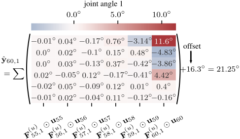
Figure 1: Example of a ReLiNet explanation on the ROBOT dataset. ReLiNet predicts ˆy60,1, which is the angle of the first robot arm joint at horizon h = 60. The matrix shows the contribution of each control variable at each time step to the predicted angle. Summing over the matrix and adding the offset yields the angle predicted by ReLiNet. ⊙ denotes element-wise multiplication.
5.2 Explainability
Table 2 summarizes the explanation results for LIME applied to LSTM, ReLiNet, and StableReLiNet for the longest prediction horizon of h = 60 across all three datasets.
From the results, we can see that ReLiNet and StableReLiNet produce an infidelity score of INF = 0.0, which suggests both of them are fully faithful. This is because their linear model at each time step acts as both a predictor and an explanation. In comparison, LIME yields non-zero infidelity scores for all datasets, which is expected for a modelagnostic explanation method. Since the infidelity metric is the NRMSE between model prediction (LSTM) and explainer prediction, we also note that the infidelity of LIME is very high for SHIP-IND and SHIP-OOD compared to the prediction errors shown in Table 1. This indicates that LIME struggles with faithfully explaining multistep prediction models.
Secondly, we found that ReLiNet and StableReLiNet achieve lower Lipschitz estimates (LIP) and therefore better robustness than LIME across all three datasets. These results demonstrate the explanation robustness of our approaches.
Additionally, we find that all three explainers yield similar simplicity scores (SIM). This is within expectations, as LIME and StableReLiNet employ mechanisms to reduce the number of significant feature importances. LIME uses a Lasso regressor as its local estimator, which enforces sparseness on its weights and therefore sparseness on the feature importances. StableReLiNet is exponentially stable and therefore provides exponentially diminishing importances to older inputs. ReLiNet does not explicitly implement a mechanism to ensure simple explanations. However, it is plausible to assume that ReLiNet is inferring this behavior from data, as most physical systems have diminishing responses to older control inputs.
Figure 1 shows an explanation generated by ReLiNet for the ROBOT dataset. The displayed matrix indicates the contribution of each control variable at each time step to the predicted joint angle. As hypothesized in the previous paragraph, ReLiNet assigns higher importance to the most recent inputs, improving explanation simplicity. Additionally, we observe that the motor attached to the first joint also has the largest impact on the corresponding angle of the joint, which matches our expectation of the actual system and accordingly indicates that ReLiNet learns physically plausible behavior.
In summary, we observe that ReLiNet yields more faithful and robust explanations compared to LIME without a reduction in explanation simplicity.
6 Conclusion
In this work, we show the competitive multistep prediction accuracy of our proposed method, ReLiNet, in comparison to LSTM, a state-of-the-art multistep prediction model, while providing explanations that are more faithful and robust than the model-agnostic explainer LIME. Additionally, we have proven that StableReLiNet, an extension of ReLiNet, is exponentially stable by definition. StableReLiNet sacrifices prediction accuracy for exponential stability performing worse than ReLiNet and LSTM but still outperforming the linear model, QLag, and switched linear model, k-LinReg.
Explainable-by-definition models are a promising direction of research for multistep prediction of dynamical systems under system-theoretic constraints. By reducing a neural network to a simpler model for each prediction, it is possible to enforce constraints on the simpler model, thereby providing provable guarantees on the neural network. We have shown this with StableReLiNet, where we reduce an LSTM to a constrained linear parameter-varying system and thereby guarantee the exponential stability of the model. Existing research on the stability of switched linear systems, such as [Lin and Antsaklis, 2009], could enable further variants of ReLiNet for different classes of stability, which might yield better tradeoffs with regards to prediction accuracy.
Acknowledgments
This research is funded by Deutsche Forschungsgemeinschaft (DFG, German Research Foundation) under Germany's Ex-
- cellence Strategy - EXC 2075 - 390740016. We acknowledge the support by the Stuttgart Center for Simulation Science (SimTech).
@inproceedings{ijcai2023p385,
  title     = {ReLiNet: Stable and Explainable Multistep Prediction with Recurrent Linear Parameter Varying Networks},
  author    = {Baier, Alexandra and Aspandi, Decky and Staab, Steffen},
  booktitle = {Proceedings of the Thirty-Second International Joint Conference on
               Artificial Intelligence, {IJCAI-23}},
  publisher = {International Joint Conferences on Artificial Intelligence Organization},
  editor    = {Edith Elkind},
  pages     = {3461--3469},
  year      = {2023},
  month     = {8},
  note      = {Main Track},
  doi       = {10.24963/ijcai.2023/385},
  url       = {https://doi.org/10.24963/ijcai.2023/385},
}
TY - CPAPER TI - ReLiNet: Stable and Explainable Multistep Prediction with Recurrent Linear Parameter Varying Networks AU - Baier, Alexandra AU - Aspandi, Decky AU - Staab, Steffen T2 - Proceedings of the Thirty-Second International Joint Conference on Artificial Intelligence, IJCAI-23 PB - International Joint Conferences on Artificial Intelligence Organization PY - 2023 SP - 3461 EP - 3469 DO - 10.24963/ijcai.2023/385 UR - https://doi.org/10.24963/ijcai.2023/385 ER -Copied
Machine-readable versions of this paper, for tools and AI agents:





