
Ensemble Reinforcement Learning in Continuous Spaces -- A Hierarchical Multi-Step Approach for Policy Training
Proceedings of the Thirty-Second International Joint Conference on Artificial Intelligence. Main Track. Pages 3514-3522.
https://doi.org/10.24963/ijcai.2023/391
Keywords
- Machine Learning: ML: Deep reinforcement learning
- Machine Learning: ML: Ensemble methods
Abstract
Actor-critic deep reinforcement learning (DRL) algorithms have recently achieved prominent success in tackling various challenging reinforcement learning (RL) problems, particularly complex control tasks with high-dimensional continuous state and action spaces. Nevertheless, existing research showed that actor-critic DRL algorithms often failed to explore their learning environments effectively, resulting in limited learning stability and performance. To address this limitation, several ensemble DRL algorithms have been proposed lately to boost exploration and stabilize the learning process. However, most of existing ensemble algorithms do not explicitly train all base learners towards jointly optimizing the performance of the ensemble. In this paper, we propose a new technique to train an ensemble of base learners based on an innovative multi-step integration method. This training technique enables us to develop a new hierarchical learning algorithm for ensemble DRL that effectively promotes inter-learner collaboration through stable inter-learner parameter sharing. The design of our new algorithm is verified theoretically. The algorithm is also shown empirically to outperform several state-of-the-art DRL algorithms on multiple benchmark RL problems.
- [Achiam, 2018] J. Achiam. Spinning Up in Deep Reinforce- ment Learning. https://github.com/openai/spinningup, 2018. Accessed: 2022-12-20. Link
- [An et al., 2021] Gaon An, Seungyong Moon, Jang-Hyun Kim, and Hyun Oh Song. Uncertainty-based offline rein- forcement learning with diversified q-ensemble. Advances in neural information processing systems, 34:7436-7447, 2021.
- [Baek et al., 2020] J. Baek, H. Jun, J. Park, H. Lee, and S. Han. Sparse variational deterministic policy gradient for continuous real time control. IEEE Transactions on Industrial Electronics, 2020.
- [Barth-Maron et al., 2018] G. Barth-Maron, M. W. Hoff- man, D. Budden, W. Dabney, D. Horgan, D. Tb, A. Mul- dal, N. Heess, and T. Lillicrap. Distributed distribu- tional deterministic policy gradients. arXiv preprint arXiv:1804.08617, 2018.
- [Bellemare et al., 2016] M. Bellemare, S. Srinivasan, G. Os- trovski, T. Schaul, D. Saxton, and R. Munos. Uni- fying count-based exploration and intrinsic motivation. Advances in neural information processing systems, 29:1471-1479, 2016.
- [Brockman et al., 2016] G. Brockman, V. Cheung, L. Pet- tersson, J. Schneider, J. Schulman, J. Tang, and W. Zaremba. Openai gym. arXiv:1606.01540, 2016.
- [Chan et al., 2019] C. Y. S. Chan, S. Fishman, J. Canny, A. Korattikara, and S. Guadarrama. Measuring the relia- bility of reinforcement learning algorithms. arXiv preprint arXiv:1912.05663, 2019.
- [Chen et al., 2017] R. Y. Chen, S. Sidor, P. Abbeel, and J. Schulman. Ucb exploration via q-ensembles. arXiv preprint arXiv:1706.01502, 2017.
- [Chen et al., 2018] G. Chen, Y. Peng, and M. Zhang. Effec- tive exploration for deep reinforcement learning via boot- strapped q-ensembles under tsallis entropy regularization. arXiv preprint arXiv:1809.00403, 2018.
- [Cobbe et al., 2021] K. W. Cobbe, J. Hilton, O. Klimov, and J. Schulman. Phasic policy gradient. In International Con- ference on Machine Learning, pages 2020-2027. PMLR, 2021.
- Ellenberger, 2018 2019]
- B. Ellenberger. Pybullet gym- perium. https://github.com/benelot/pybullet-gym, 2018- 2019. Accessed: 2022-12-20. Link
- [Fujimoto et al., 2018] S. Fujimoto, H. Hoof, and D. Meger. Addressing function approximation error in actor-critic methods. In International Conference on Machine Learn- ing, pages 1587-1596. PMLR, 2018.
- [Haarnoja et al., 2018] T. Haarnoja, A. Zhou, P. Abbeel, and S. Levine. Soft actor-critic: Off-policy maximum entropy deep reinforcement learning with a stochastic actor. In In- ternational conference on machine learning, pages 1861- 1870. PMLR, 2018.
- [Hasselt et al., 2016] H. Van Hasselt, A. Guez, and D. Sil- ver. Deep reinforcement learning with double q-learning. In Proceedings of the AAAI conference on artificial intel- ligence, volume 30, 2016.
- [Huang et al., 2017] Z. Huang, S. Zhou, B. Zhuang, and X. Zhou. Learning to run with actor-critic ensemble. arXiv preprint arXiv:1712.08987, 2017.
- [Ibarz et al., 2021] J. Ibarz, J. Tan, C. Finn, M. Kalakrishnan, P. Pastor, and S. Levine. How to train your robot with deep reinforcement learning: lessons we have learned. The International Journal of Robotics Research, 40(4-5):698- 721, 2021.
- [Januszewski et al., 2021] P. Januszewski, M. Olko, M. Królikowski, J. Światkowski, M. Andrychowicz, L. Kuciński, and P. Miloś. Continuous control with ensemble deep deterministic policy gradients. arXiv preprint arXiv:2111.15382, 2021.
- [Kurutach et al., 2018] T. Kurutach, I. Clavera, Y. Duan, A. Tamar, and P. Abbeel. Model-ensemble trust-region policy optimization. arXiv preprint arXiv:1802.10592, 2018.
- [Lai et al., 2020] Kwei-Herng Lai, Daochen Zha, Yuening Li, and Xia Hu. Dual policy distillation. arXiv preprint arXiv:2006.04061, 2020.
- [Lakshminarayanan et al., 2016] B. Lakshminarayanan, A. Pritzel, and C. Blundell. Simple and scalable predictive uncertainty estimation using deep ensembles. arXiv preprint arXiv:1612.01474, 2016.
- [Lee et al., 2021] K. Lee, M. Laskin, A. Srinivas, and P. Abbeel. Sunrise: A simple unified framework for en- semble learning in deep reinforcement learning. In Inter- national Conference on Machine Learning, pages 6131- 6141. PMLR, 2021.
- [Lillicrap et al., 2015] T. P. Lillicrap, J. J. Hunt, A. Pritzel, N. Heess, T. Erez, Y. Tassa, D. Silver, and D. Wier- stra. Continuous control with deep reinforcement learning. arXiv preprint arXiv:1509.02971, 2015.
- [Liu et al., 2021] R. Liu, F. Nageotte, P. Zanne, M. de Math- elin, and B. Dresp-Langley. Deep reinforcement learning for the control of robotic manipulation: a focussed mini- review. Robotics, 10(1):22, 2021.
- [Mnih et al., 2016] V. Mnih, A. P. Badia, M. Mirza, A. Graves, T. Lillicrap, T. Harley, D. Silver, and K. Kavukcuoglu. Asynchronous methods for deep rein- forcement learning. In International conference on ma- chine learning, pages 1928-1937. PMLR, 2016.
- [Osband and Roy, 2017] I. Osband and B. Van Roy. Why is posterior sampling better than optimism for reinforcement learning? In International conference on machine learn- ing, pages 2701-2710. PMLR, 2017.
- [Osband et al., 2016] I.
- Osband, C. Blundell, A. Pritzel, and B. Van Roy. Deep exploration via bootstrapped dqn. Advances in neural information processing systems, 29:4026-4034, 2016.
- [Osband et al., 2018] I.
- Osband, J. Aslanides, and A. Cas- sirer. Randomized prior functions for deep reinforcement learning. arXiv preprint arXiv:1806.03335, 2018.
- [Paine et al., 2020] T. L. Paine, C. Paduraru, A. Michi, C. Gulcehre, K. Zolna, A. Novikov, Z. Wang, and N. de Freitas. Hyperparameter selection for offline re- inforcement learning. arXiv preprint arXiv:2007.09055, 2020.
- [Plappert et al., 2017] M. Plappert, R. Houthooft, P. Dhari- wal, S. Sidor, R. Y. Chen, X. Chen, T. Asfour, P. Abbeel, and M. Andrychowicz. Parameter space noise for explo- ration. arXiv preprint arXiv:1706.01905, 2017.
- [Reizinger and Szemenyei, 2020] P. Reizinger and M. Sze- menyei. Attention-based curiosity-driven exploration in deep reinforcement learning. In ICASSP 2020-2020 IEEE International Conference on Acoustics, Speech and Signal Processing (ICASSP), pages 3542-3546. IEEE, 2020.
- [Schulman et al., 2015] J. Schulman, N. Heess, T. Weber, and P. Abbeel. Gradient estimation using stochastic com- putation graphs. Advances in Neural Information Process- ing Systems, 28:3528-3536, 2015.
- [Schulman et al., 2017] J. Schulman, F. Wolski, P. Dhariwal, A. Radford, and O. Klimov. Proximal policy optimization algorithms. arXiv preprint arXiv:1707.06347, 2017.
- [Scieur et al., 2017] D. Scieur, V. Roulet, F. Bach, and A. d'Aspremont. Integration methods and accelerated op- timization algorithms. arXiv preprint arXiv:1702.06751, 2017.
- [Shani et al., 2020] L. Shani, Y. Efroni, and S. Mannor. Adaptive trust region policy optimization: Global conver- gence and faster rates for regularized mdps. In Proceed- ings of the AAAI Conference on Artificial Intelligence, vol- ume 34, pages 5668-5675, 2020.
- [Silver et al., 2014] D. Silver, G. Lever, N. Heess, T. Degris, D. Wierstra, and M. Riedmiller. Deterministic policy gra- dient algorithms. In International conference on machine learning, pages 387-395. PMLR, 2014.
- [Wang et al., 2020] C. Wang, Y. Wu, Q. Vuong, and K. Ross. Striving for simplicity and performance in off-policy drl: Output normalization and non-uniform sampling. In Inter- national Conference on Machine Learning, pages 10070- 10080. PMLR, 2020.
- [Wiering and Hasselt, 2008] M. A. Wiering and H. Van Has- selt. Ensemble algorithms in reinforcement learning. IEEE Transactions on Systems, Man, and Cybernetics, Part B (Cybernetics), 38(4):930-936, 2008.
- [Wu et al., 2017] Y. Wu, E. Mansimov, R. B. Grosse, S. Liao, and J. Ba. Scalable trust-region method for deep reinforcement learning using kronecker-factored approxi- mation. Advances in neural information processing sys- tems, 30:5279-5288, 2017.
- [Zhelo et al., 2018] O. Zhelo, J. Zhang, L. Tai, M. Liu, and W. Burgard. Curiosity-driven exploration for mapless nav- igation with deep reinforcement learning. arXiv preprint arXiv:1804.00456, 2018.
References were extracted automatically from the PDF and may contain errors.
Full text extracted automatically from the PDF; figures, tables and equations may differ. The PDF is the version of record.
1 Introduction
Deep reinforcement learning (DRL) is a booming field of research in machine learning with diverse real-world applications [Ibarz et al., 2021]. In recent years, many model-free DRL algorithms achieved cutting-edge performance in tackling various continuous reinforcement learning (RL) problems, including complex control tasks with high-dimensional state and action spaces [Liu et al., 2021]. These algorithms can effectively train deep neural networks (DNNs) to precisely model high-quality control policies and are the central focus of this paper 1 .
1 A long version of this paper with all referenced appendices can be accessed through https://arxiv.org/abs/2209.14488.
Despite of widely reported success, a majority of existing actor-critic DRL algorithms, such as DDPG [Lillicrap et al., 2015], SAC [Haarnoja et al., 2018] and PPO [Schulman et al., 2017], still suffer from some major limitations. Specifically, existing research works showed that the algorithm performance is highly sensitive to hyper-parameter settings and can vary substantially in different algorithm runs [Paine et al., 2020]. Ineffective exploration is often considered as a major cause for the poor learning stability [Chan et al., 2019], often resulting in overfitting and premature convergence to poor local optima [Kurutach et al., 2018].
Rather than relying on one learner (or DRL agent), an ensemble of base learners can be jointly utilized to boost exploration and stabilize the learning process [Osband et al., 2016; Osband and Roy, 2017]. For example, the ensemble deep deterministic policy gradient (ED2) algorithm is a newly developed ensemble DRL method [Januszewski et al., 2021] that trains multiple DNN policies simultaneously using a shared experience replay buffer (ERB), similar to several previously proposed parallel DRL algorithms [Barth-Maron et al., 2018; Mnih et al., 2016]. ED2 features a unique mixture of multiple well-studied tricks, including temporally-extended deep exploration, double Q-bias reduction, and target policy smoothing [Osband et al., 2016; Osband and Roy, 2017; Hasselt et al., 2016; Fujimoto et al., 2018]. It was reported to outperform state-of-the-art ensemble DRL algorithms such as SUNRISE [Lee et al., 2021] on several difficult Mujoco benchmark control problems.
As far as we know, many existing ensemble DRL algorithms are designed to train each base learner individually. For example, in ED2, every base learner trains its own DNN policy using its own critic, with the aim to improve its own performance without considering the impact of the trained policy on the ensemble. While sharing the same ERB, policy training is conducted largely independently by all base learners. This is shown to promote healthy exploration in [Januszewski et al., 2021]. However, there is no guarantee that the base learners will collaborate effectively such that the ensemble as a whole can achieve desirable performance.
To address this limitation, we propose a new hierarchical approach for training base learners in this paper. Specifically, we follow ED2 for low-level training of DNN policies, which will be performed concurrently by all base learners. In the meantime, we construct a global critic, which is trained constantly to predict the performance of the ensemble. Guided by the global critic, high-level training of DNN policies will be performed regularly to strengthen cooperation among all the base learners.
Since the ensemble is not used directly to collect statetransition samples from the learning environment, we must make sure that high-level training of the ensemble is not performed on out-of-distribution data obtained by individual base learners. In view of this, it is important to encourage inter-learner parameter sharing so that the DNN policy trained by one base learner can contribute directly to the training of DNN policies by other base learners. For this purpose, we develop a new technique in this paper for high-level training of policies based on the multi-step integration methods [Scieur et al., 2017].
Our high-level policy training technique is theoretically justified as it guarantees stability for a wide range of optimization problems. Meanwhile, it can be shown analytically that, for all base learners, their trained linear parametric policies (a special and important technique for policy approximation) are expected to behave more consistently as the ensemble through high-level policy training, encouraging interlearner collaboration and alleviating the data distribution issue.
Driven by the hierarchical policy training method, we develop a new ensemble DRL algorithm called the hierarchical ensemble deep deterministic policy gradient (HED) in this paper. Experimental evaluation of HED has been conducted on a range of benchmark control problems, including the widely used Mujoco control tasks as well as the less popular and potentially more challenging PyBullet control problems. Our experiments clearly show that HED can outperform ED2, SUNRISE and several cutting-edge DRL algorithms on multiple benchmark problems.
2 RelatedWork
Similar to ED2, HED trains an ensemble of policies using an off-policy DRL algorithm to leverage on the algorithm's advantages in sample efficiency. Recently, several off-policy DRL algorithms have been developed successfully for RL in continuous spaces, including DDPG [Lillicrap et al., 2015], SAC [Haarnoja et al., 2018], TD3 [Fujimoto et al., 2018], and SOP [Wang et al., 2020]. These algorithms introduce a variety of tricks to stabilize the learning process. For example, TD3 extends the idea of double Q-network [Hasselt et al., 2016] to a new double-Q bias reduction technique, which can effectively prevent over-optimistic training of DNN policies. In addition, empirical evidence showed that the learning process becomes more stable when the actor and critic in TD3 are trained with different frequencies [Fujimoto et al., 2018; Cobbe et al., 2021]. The base learners in our HED ensemble will adopt these tricks.
The recent literature also provides some new tricks to stabilize learning. Specifically, various trust-region methods have been developed to prevent negative behavioral changes during policy training [Kurutach et al., 2018; Schulman et al., 2015; Shani et al., 2020; Wu et al., 2017; Schulman et al., 2017]. Meanwhile, entropy regularization techniques prohibit immature convergence of the trained policies and ensure prolonged profitable exploration [Chen et al., 2018; Haarnoja et al., 2018]. However, these techniques are mainly applied to stochastic policies while we aim at learning an ensemble of deterministic policies. Previous research showed that deterministic policies can often be trained more efficiently than stochastic policies using the reparameterization trick [Fujimoto et al., 2018; Silver et al., 2014; Baek et al., 2020].
The stability of a DRL algorithm depends critically on how the learner explores its environment. Besides the entropy regularization methods, curiosity metrics are popularly employed to encourage a learner to explore rarely visited states during RL [Reizinger and Szemenyei, 2020; Zhelo et al., 2018]. Meanwhile, many previous studies embraced the optimum in the face of uncertainty (OFU) principle to design bonus rewards for actions with high potentials, thereby promoting exploration in promising areas of the learning environment [Bellemare et al., 2016]. One good example is the UCB exploration technique developed in [Chen et al., 2017; Lee et al., 2021]. However, in [Januszewski et al., 2021], this technique was shown to be less effective than the bootstrap with random initialization trick adopted in ED2. Temporallyextended exploration on RL problems with continuous actions can also be achieved by adding a small amount of noise to DNN weights [Plappert et al., 2017]. This is directly related to the posterior sampling methods that are often used to select the best actions among a statistically plausible set of sampled actions [Osband et al., 2018].
Following the OFU principle, deep ensembles have been recently proposed to approximate Bayesian posteriors with high accuracy and efficiency [Lakshminarayanan et al., 2016]. They are subsequently exploited to approach deep exploration for reliable RL [Osband et al., 2016]. Several issues have been investigated under the context of ensemble DRL. For instance, the diversity of base learners is essential to the performance of the ensemble. To encourage diversity, either different DRL algorithms or the same algorithm with differed hyper-parameter settings have been adopted to train base learners [Huang et al., 2017; Wiering and Hasselt, 2008]. The training of each base learner can also be supported by an ensemble of critics [An et al., 2021]. Meanwhile, inter-learner collaboration can be encouraged by asking one learner to imitate the behavior of the other learner that is expected to perform better in the ensemble [Lai et al., 2020]. This idea gives rise to the DPD-PPO algorithm that only supports an ensemble with two learners. Some experiment results that compare the performance of DPD-PPO with HED can be found in Appendix F.
As far as we know, few existing ensemble DRL algorithms in the literature have ever studied the important issue on how to effectively train all base learners to jointly improve the ensemble performance. This issue will be explored in-depth with the newly developed HED algorithm in this paper.
3 Background
An RL problem is modeled as a Markov Decision Process (MDP) (S, A, R, P, γ, p0), where S and A refer respectively to the continuous multi-dimensional state space and action space. P stands for the state-transition model that governs the probability of reaching any state st+1 ∈ S at timestep t + 1 upon performing any action at ∈ A in state st ∈ S at timestep t, with t ∈ Z+. Additionally, γ ∈ [0, 1) is the discount factor, R is the reward function, and p0 captures the initial state distribution.
To solve any RL problem described above, we aim to learn an optimal deterministic ensemble policy πe ∗ (s) that maps any state input s ∈ S to an action vector a ∈ A so as to maximize the cumulative rewards defined below
where τ = [(st, at, rt, st+1)]∞t=1 contains a series of consecutive state-transition samples and is called a episode, which can be obtained by following the ensemble policy πe , and rt = R(st, at) is the immediate reward received at timestep t in τ . For an ensemble with N base learners where each base learner Li, 1 ≤ i ≤ N, maintains its own deterministic base policy πi , the action output of πe is jointly determined by all the base policies according to
In order to train an ensemble to maximize the cumulative rewards, our baseline algorithm ED2 uses randomly selected base learners to sample a series of episodes {τi}, which will be stored in the shared ERB. At regular time intervals, a minibatch of state-transition samples will be retrieved from the ERB. Every base learner Li will then use the retrieved minibatch to train its own actor πi and critic Qi individually. In other words, a base learner manages two separate DNNs, one models the deterministic policy πi and the other approximates the Q-function Qi of πi . A base learner uses an existing actorcritic RL algorithm to train the two DNNs. In this paper, we choose TD3 for this purpose due to its proven effectiveness, high popularity and stable learning behavior [Fujimoto et al., 2018].
4 Hierarchical Ensemble Deep Deterministic Policy Gradient
The pseudo-code of the HED algorithm is presented in Algorithm 1. HED follows many existing works including ED2 [Osband et al., 2016; Januszewski et al., 2021] to achieve temporally-extended exploration through bootstrapping with random initialization of DNN policies. As clearly shown in [Januszewski et al., 2021], this exploration technique is more effective than UCB and parameter randomization methods. Different from ED2 which completely eliminates the necessity of adding small random noises to the deterministic action outputs from the DNN policies, we keep a small level of action noise 2 while using any chosen policy to explore the learning environment. We found empirically that this ensures coherent exploration, similar to [Osband et al., 2016], while making the testing performance of the trained policies more stable.
2 The noise is sampled from the Normal distribution independently for each dimension of the action vector. The variance of the normal distribution is fixed at 0.01 during the learning process.
Different from ED2 and other ensemble algorithms for RL in continuous spaces, HED trains DNN policies at two separate levels. The low-level training of πi and Qi by each base learner Li is essentially the same as ED2 and TD3. Specifically, for any base learner Li, i ∈ {1, . . . ,N}, Qi is trained by Li to minimize MSEi below
where ϕi represents the trainable parameters of the DNN that approximates Qi . B is the random mini-batch retrieved from the ERB. ˆQik with k = 1, 2 stands for the two target Qnetworks of Li that together implement the double-Q bias reduction mechanism proposed in [Fujimoto et al., 2018]. Additionally, ϵ is a random noise sampled from a Normal distribution with zero mean and small variance 3 . Using the trained Qi , the trainable parameters θi of the DNN that models policy πi is further updated by Li along the policy gradient direction computed below
Besides the above, HED constantly trains a separate highlevel Q-function Qe to predict the performance of the ensemble policy πe . Guided by the trained Qe , high-level policy training is conducted regularly to update policy πi of all base learners so as to enhance their cooperation and performance.
A new multi-step technique is developed in HED to enable inter-learner parameter sharing during high-level policy training. To implement this technique, we keep track of a list of bootstrap policy parameters for the multi-step training process. More details can be found in the following subsection. Theoretical justifications regarding the usefulness of the multi-step approach are also provided below.
4.1 Multi-Step High-Level Policy Training
In addition to Qi for each base learner Li, i ∈ {1, . . . ,N}, HED maintains a separate Q-network to approximate Qe of the ensemble policy πe . Similar to (2), HED trains this central Q-network towards minimizing MSEe below
with ϕe representing the trainable parameters of the central Q-network. ˆQe stands for the corresponding target Qnetwork that stabilizes the training process. For simplicity, we do not add random noise ϵ in (2) to the action outputs produced by the ensemble policy πe in (4). Furthermore, following [Hasselt et al., 2016], one target Q-network instead of
3 The variance for sampling ϵ is kept at a very small level of 0.01 in the experiments.
Algorithm 1 The pseudo-code of the HED algorithm.
Input: Ensemble size N; initial policy networks πiθi and Q-networks Qiϕi for i ∈ {1, . . . ,N}; ERB; ensemble Qnetwork Qeϕe ; target Q-networks for each base learner and the ensemble
Output: Trained ensemble policy πe
While total number of sampled trajectories < max number of trajectories:
Randomly sample i ∈ {1, . . . , N}
While the current trajectory does not terminate:
Use πi to perform the next action
Store sampled state-transition in ERB
Track number of steps sampled before critic training If time for critic training:
For number of steps sampled:
Sample a mini-batch B from ERB
Train Qiϕi for i ∈ {1, . . . ,N} using (2)
Train Qeϕe using (4)
If time for low-level policy training:
Train πiθi for i ∈ {1, . . . ,N} using (3)
If time for high-level policy training:
Set bootstrap list {xj}2j=0 for each base learner
For a fraction of sampled steps:
Train πiθi for i ∈ {1, . . . ,N} using (9)
Append trained θi for i ∈ {1, . . . ,N} to the bootstrap lists of each base learner for the next step of high-level policy training
two is adopted in (4) to facilitate the training of Qe . Building on the trained Qe , we can calculate the ensemble policy gradient with respect to θi of every base learner Li as follows
with
according to (1). I stands for the m × m identity matrix where m is the dimension of the action vector. One straightforward approach for high-level policy training is to update θi of every base learner Li in the direction of (5). However, using (5) alone may not encourage any base learner Li to behave consistently with the ensemble (see Proposition 2). Consequently, high-level training of the ensemble policy may be performed on the out-of-distribution state-transition samples collected by the base learners, affecting the training effectiveness. Furthermore, ensembles are used mainly for temporally-extended exploration in the literature. Except [Lai et al., 2020], the learning activity of one base learner may only indirectly influence the learning activities of other base learners through the shared ERB. Base learners do not explicitly share their learned policy parameters to strengthen inter-learner cooperation and boost the learning process.
To address this limitation, we propose to promote interlearner parameter sharing during high-level policy training, in order to achieve a desirable balance between exploration and inter-learner cooperation. Specifically, in addition to (5), we randomly select two base learners Lp and Lq and use their policy parameters to guide the training of policy πi of any base learner Li. In comparison to selecting one base learner, this allows more base learners to have the opportunity to share their parameters with the base learner Li during policy training. It is also possible to recruit more than two base learners. However, in this case, it is mathematically challenging to derive stable learning rules for high-level policy training.
Motivated by the above discussion, a search through the literature leads us to the linear multi-step integration methods recently analyzed in [Scieur et al., 2017]. Consider a simple gradient flow equation below
where θ0 i refers to the initial policy parameter of base learner Li. If J(πe ) is strongly concave and Lipschitz continuous, the solution of (6) allows us to obtain the optimal policy parameters θ∗ i when x(t) approaches to ∞. Since J(πe ) is not strongly concave for most of real-world RL problems, x(t) in practice may only converge to a locally optimal policy, which is common among majority of the policy gradient DRL algorithms. Therefore high-level training of policy πe and hence πi can be approached by numerically solving (6). This can be achieved through a linear µ-step method shown below
where ρj , σj ∈ R are the pre-defined coefficients of the multistep method and h is the learning rate. Clearly, each new point xk+µ produced by the µ-step method is a function of the preceding µ points. In this paper, we specifically consider the case when µ = 3. Meanwhile, let
where p and q are the randomly generated indices of two base learners and i is the index of the base learner whose policy πi is being trained by the µ-step method. Through this way, the training of policy πi is influenced directly by base learners Lp and Lq through explicit inter-learner parameter sharing. xi(i ≥ 3) in (7) represents the trained policy parameters of πi in subsequent training steps.
Although (7) allows us to use ∇θp J(πe ) and ∇θq J(πe ) to train θi, they do not seem necessary for inter-learner parameter sharing. To simplify (7), we set σ0 = σ1 = 0 and σ2 = 1. Hence only g(xk+2), which is the ensemble policy gradient with respect to policy πi in (5), is used to train πi . With this simplification, we derive the new learning rule for high-level policy training below
To implement (9) in HED, before high-level policy training, every base learner Li must set up a bootstrap list of policy parameters {x0 = θp, x1 = θq, x2 = θi}. After the k-th training step (k ≥ 0) based on (9), Li appends the trained θi as xk+3 to the bootstrap list, which will be utilized to train πi in the subsequent training steps. Reliable use of (9) demands for careful parameter settings of ρ0, ρ1, ρ2 and h. Relevant theoretical analysis is presented below.
4.2 Theoretical Analysis
In this subsection, a theoretical analysis is performed first to determine suitable settings of ρ0, ρ1, ρ2 and h for stable highlevel policy training through (9). To make the analysis feasible, besides the strongly concave and Lipschitz continuous conditions, we further assume that
where A is a positive definite matrix whose eigenvalues are bounded positive real numbers. θ∗ i stands for the globaloptimal (or local-optimal) policy parameters. Many strongly concave functions satisfy this assumption [Scieur et al., 2017]. Meanwhile, the attraction basin of the local optimum of many multi-modal optimization problems often satisfies this assumption too. Using this assumption, we can derive Proposition 1 below.
Proposition 1. Upon using (9) to numerically solve (6), the following conditions must be satisfied for xk to converge to θ∗ i as k approaches to∞:
3. h is reasonably small such that 0 ≤ λh < 2-4ρ0, where λ can take any real value between the smallest and the largest eigenvalues of the positive definite matrix A in (10).
The proof of Proposition 1 can be found in Appendix A. Proposition 1 provides suitable parameter settings for (9) and justifies its stable use for high-level policy training. We next show that (9) is also expected to make base learners behave more consistently with the ensemble, without affecting the behavior of the trained ensemble, when ρ0 is sufficiently small. Consider specifically that each base learner Li trains a linear parametric policy of the form:
where Φ(s) represents the state feature vector with respect to any input state s. For simplicity, we study the special case of scalar actions. However, the analysis can be easily extended to high-dimensional action spaces. Meanwhile, we use Sin() and Mul() to represent respectively the action output of a policy trained for one iteration on the same state s by using either the single-step method or the multi-step method in (9). The single-step method can be considered as a special case of the multi-step method with ρ2 = -1 and ρ0 = ρ1 = 0. Using these notations, Proposition 2 is presented below.
Proposition 2. When each base learner Li, i ∈ {1, . . . ,N}, trains its linear parametric policy πi with policy parameters θi on any state s ∈ S and when 0 < ρ0 < 13 ,
where the expectations above are taken with respect to any randomly selected p, q ∈ {1, . . . , N} in (8).
Proposition 2 indicates that multi-step training in (9) is expected to reduce the difference between the action output of any base learner and that of the ensemble. Meanwhile the amount of action changes applied to πe remains identical to the single-step method. Therefore, using the multi-step policy training method developed in this section helps to enhance consistent behaviors among all base learners of the ensemble.
5 Experiment
This section presents the experimental evaluation of HED, in comparison to several state-of-the-art DRL algorithms. The experiment setup is discussed first. Detailed experiment results are further presented and analyzed.
5.1 Experiment Setting
We implement HED based on the high-quality implementation of TD3 provided by the publicly available OpenAI Spinning Up repository [Achiam, 2018]. We also follow closely the hyper-parameter settings of TD3 recommended in [Fujimoto et al., 2018] to build each base learner of HED. Specifically, a fully connected MLP with two hidden layers of 256 ReLU units is adopted to model all policy networks and Q-networks. Similar to [Januszewski et al., 2021; Lee et al., 2021], HED employs 5 base learners, i.e., N = 5. Each base learner has its own policy network and Q-network. Meanwhile, HED maintains and trains a separate ensemble Q-network with the same network architecture design.
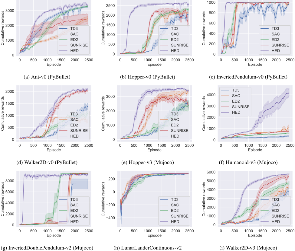
Each base learner trains its Q-network and also conducts the low-level training of the policy network repeatedly whenever HED collects 50 consecutive state-transition samples from the learning environment. Meanwhile, high-level policy training as well as the training of the ensemble Q-network is performed immediately after HED samples a full episode. HED adopts a separate Adam optimizer with the fixed learning rate of 1e-3 to train each Q-network and policy network. Furthermore, ρ0 in (9) is set to 0.0001 for the main experiment results reported in Figure 1. The mini-batch size |B| is set to 256, following existing research [Januszewski et al., 2021; Fujimoto et al., 2018] without any fine-tuning.
HED is compared against four state-of-the-art DRL algorithms, including two Ensemble DRL algorithms, i.e., ED2 [Januszewski et al., 2021] and SUNRISE [Lee et al., 2021]), and two widely used off-policy DRL algorithms, i.e., SAC [Haarnoja et al., 2018] and TD3 [Fujimoto et al., 2018]. We evaluate their performance on 9 challenging continuous control benchmark problems, including four PyBullet benchmark problems [Ellenberger, 2018 2019] (i.e., Ant-v0, Hopper-v0, InvertedPendulum-v0, and Walker2D-v0), five Mujoco control tasks (i.e., Hopper-v3, Humanoid-v3, InvertedDoublePendulum-v0, and Walker2Dv3), and LunarLanderContinuous-v2 provided by OpenAI
| Benchmark problems | TD3 | SAC | ED2 | SUNRISE | HED |
|---|---|---|---|---|---|
| Ant-v0 (PyBullet) | 3246.82±184.03 | 2453.23±523.96 | 3285.06±183.98 | 2425.93±1120.12 | 3370.12±179.95 |
| Hopper-v0 (PyBullet) | 2051.68±567.12 | 2126.43±165.58 | 2284.41±203.79 | 1585.17±761.78 | 2530.85±277.26 |
| InvertedPendulum-v0 (PyBullet) | 958.15±33.38 | 995.69±12.94 | 1000.00±0.00 | 995.69±5.27 | 1000.00±0.00 |
| Walker2D-v0 (PyBullet) | 1379.56±394.77 | 774.19±281.45 | 1082.42±312.4 | 2012.15±148.73 | 2109.49±116.79 |
| Hopper-v3 (Mujoco) | 2374.47±721.68 | 3306.01±410.28 | 2361.13±1101.71 | 2427.12±622.42 | 3396.9±249.11 |
| Humanoid-v3 (Mujoco) | 321.1±225.3 | 1151.49±598.54 | 596.57±113.03 | 756.66±143.06 | 4223.77±1119.55 |
| InvertedDoublePendulum-v2 (Mujoco) | 7417.5±3694.8 | 9355.67±11.04 | 9323.89±22.15 | 9351.58±22.15 | 9144.38±327.28 |
| LunarLanderContinuous-v2 | 275.69±5.99 | 277.67±3.44 | 275.7±7.2 | 282.84±1.99 | 286.29±0.8 |
| Walker2D-v3 (Mujoco) | 3805.88±1402.27 | 4240.35±694.64 | 4750.82±530.3 | 5510.83±669.98 | 5778.84±133.15 |
Gym [Brockman et al., 2016]. In literature, PyBullet benchmarks are often considered to be more challenging than Mujoco benchmarks. Hence we decide to evaluate the performance of HED on both PyBullet and Mujoco benchmarks. The maximum episode length for each benchmark is fixed to 1000 timesteps. Each algorithm runs independently with 10 random seeds on all benchmarks. Besides the hyperparameter settings of HED highlighted above, more detailed hyper-parameter settings of all competing algorithms have been summarized in Appendix C.
5.2 Experiment Result
Performance Comparison
Table 1 presents the average cumulative rewards obtained by the policy networks (or policy ensembles for ensemble DRL algorithms) trained by all the competing algorithms across the same number of sampled episodes with respect to each benchmark. As evidenced in the table, HED achieved consistently the best performance 4 on most of the benchmark problems except InvertedDoublePendulum. Meanwhile, on InvertedDoublePendulum, HED achieved very competitive performance with at least 97% of the highest cumulative rewards reached by the best performing competing algorithms. Furthermore, on some problems such as Humanoid-v3, HED outperformed the lowest performing algorithm by up to 1200% and the algorithm with the second highest performance by up to 600%. Besides the results on the average cumulative rewards, the maximum cumulative rewards achieved by each algorithm have been reported in Appendix F for all experimented benchmarks.
In addition to Table 1, we also compared the learning curves of all the competing algorithms in Figure 1. As demonstrated in this figure, by explicitly strengthening interlearner collaboration, HED converges clearly faster and is more stable during the learning process than other competing algorithms. Specifically, on several benchmark problems, such as Hopper-v0, InvertedPendulum-v0, Hopper-v3, InvertedDoublePendulum, and Walker2D-v3, HED achieved significantly higher sample efficiency and lower variations in learning performance across 10 independent runs. In comparison to other ensemble DRL algorithms, the learning curves of HED also appear to be smoother on several benchmark problems, such as Hopper-v0 and Walker2D-v3, suggesting that HED can achieve highly competitive stability during learning.
Performance Impact of ρ0
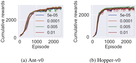
To investigate the performance impact of ρ0, we tested 4 different settings of ρ0, ranging from 5e-05 to 0.01, on the Ant-v0 and Hopper-v0 problems (similar observations can be found on other benchmark problems and are omitted in this paper). The learning curves are plotted in Figure 2. It is witnessed in the figure that the impact of different ρ0 on the final performance appears to be small as long as ρ0 is reasonably small according to Proposition 1.
4 HED significantly outperformed ED2 on most benchmark problems, thanks to its use of the proposed high-level policy training technique.
Ablation Study on High-Level Policy Training Techniques
High-level policy training can be conducted repeatedly whenever HED obtains either a full sampled episode or a fixed number of consecutive state-transition samples (e.g., samples collected from 50 consecutive timesteps). To understand which approach is more effective, experimental comparisons have been conducted in Appendix D with detailed performance results. According to the experiment results in Appendix D, episodic learning can produce more stable learning behavior and also makes HED converge faster with higher performance.
We also compared HED with its variation that performs high-level policy training by using the single-step method in (5) instead of the multi-step method in (9). Detailed experiment results can be found in Appendix E. Our experiment results confirm that multi-step training in (9) enables HED to achieve significantly faster convergence and learning stability than using the conventional single-step training technique in (5). Hence, by explicitly sharing learned policy parameters among base learners in an ensemble through (9), HED can effectively enhance inter-learner collaboration and boost the learning process.
6 Conclusions
In this paper, we conducted in-depth study of ensemble DRL algorithms, which have achieved cutting-edge performance on many benchmark RL problems in the recent literature. Different from existing research works that rely mainly on each base learner of an ensemble to train its policy network individually, we developed a new HED algorithm to explore the potential of training all base learners in a hierarchical manner in order to promote inter-learner collaboration and improve the collective performance of an ensemble of trained base learners. Specifically, we adopted existing ensemble DRL algorithms such as ED2 to perform low-level policy training. Meanwhile, a new multi-step training technique was developed for high-level policy training in HED to facilitate direct inter-learner parameter sharing. Both theoretical and empirical analysis showed that the HED algorithm can achieve stable learning behavior. It also outperformed several state-of-the-art DRL algorithms on multiple benchmark RL problems.
@inproceedings{ijcai2023p391,
  title     = {Ensemble Reinforcement Learning in Continuous Spaces -- A Hierarchical Multi-Step Approach for Policy Training},
  author    = {Chen, Gang and Huang, Victoria},
  booktitle = {Proceedings of the Thirty-Second International Joint Conference on
               Artificial Intelligence, {IJCAI-23}},
  publisher = {International Joint Conferences on Artificial Intelligence Organization},
  editor    = {Edith Elkind},
  pages     = {3514--3522},
  year      = {2023},
  month     = {8},
  note      = {Main Track},
  doi       = {10.24963/ijcai.2023/391},
  url       = {https://doi.org/10.24963/ijcai.2023/391},
}
TY - CPAPER TI - Ensemble Reinforcement Learning in Continuous Spaces -- A Hierarchical Multi-Step Approach for Policy Training AU - Chen, Gang AU - Huang, Victoria T2 - Proceedings of the Thirty-Second International Joint Conference on Artificial Intelligence, IJCAI-23 PB - International Joint Conferences on Artificial Intelligence Organization PY - 2023 SP - 3514 EP - 3522 DO - 10.24963/ijcai.2023/391 UR - https://doi.org/10.24963/ijcai.2023/391 ER -Copied
Machine-readable versions of this paper, for tools and AI agents:





