
Incremental and Decremental Optimal Margin Distribution Learning
Proceedings of the Thirty-Second International Joint Conference on Artificial Intelligence. Main Track. Pages 3523-3531.
https://doi.org/10.24963/ijcai.2023/392
Keywords
- Machine Learning: ML: Incremental learning
- Machine Learning: ML: Classification
Abstract
Incremental and decremental learning (IDL) deals with the tasks where new data arrives sequentially as a stream or old data turns unavailable continually due to the privacy protection. Existing IDL methods mainly focus on support vector machine and its variants with linear-type loss. There are few studies about the quadratic-type loss, whose Lagrange multipliers are unbounded and much more difficult to track. In this paper, we take the latest statistical learning framework optimal margin distribution machine (ODM) which involves a quadratic-type loss due to the optimization of margin variance, for example, and equip it with the ability to handle IDL tasks. Our proposed ID-ODM can avoid updating the Lagrange multipliers in an infinite range by determining their optimal values beforehand so as to enjoy much more efficiency. Moreover, ID-ODM is also applicable when multiple instances come and leave simultaneously. Extensive empirical studies show that ID-ODM can achieve 9.1x speedup on average with almost no generalization lost compared to retraining ODM on new data set from scratch.
- [Boyd and Vandenberghe, 2004] Stephen P. Boyd and Lieven Vandenberghe. Convex Optimization. Cambridge University Press, Cambridge, United Kingdom, 2004.
- [Cauwenberghs and Poggio, 2000] Gert Cauwenberghs and Tomaso A. Poggio. Incremental and decremental support vector machine learning. In Advances in Neural Infor- mation Processing Systems, pages 409-415, Denver, CO, 2000.
- [Chen et al., 2023] Haiyan Chen, Ying Yu, Yizhen Jia, and Bin Gu. Incremental learning for transductive support vec- tor machine. Pattern Recognition, 133:10982, 2023.
- [Cherubin et al., 2021] Giovanni Cherubin, Konstantinos Chatzikokolakis, and Martin Jaggi. Exact optimization of conformal predictors via incremental and decremental learning. In Proceedings of the 38th International Con- ference on Machine Learning, pages 1836-1845, virtual, 2021.
- [Cortes and Vapnik, 1995] Corinna Cortes and Vladimir Vapnik. Support-vector networks. Machine Learning, 20(3):273-297, 1995.
- [Ertekin et al., 2007] Seyda Ertekin, Jian Huang, Léon Bot- tou, and C. Lee Giles. Learning on the border: active learn- ing in imbalanced data classification. In Proceedings of the 16th ACM Conference on Information and Knowledge Management, pages 127-136, Lisbon, Portugal, 2007.
- [Gâlmeanu and Andonie, 2022] Honorius Gâlmeanu and Razvan Andonie. Weighted incremental-decremental support vector machines for concept drift with shifting window. Neural Networks, 152(5):528-541, 2022.
- [Gao and Zhou, 2013] Wei Gao and Zhi-Hua Zhou. On the doubt about margin explanation of boosting. Artificial In- telligence, 203:1-18, 2013.
- [Golub and Van Loan, 1983] Gene H. Golub and Charles F. Van Loan. Matrix Computations. Johns Hopkins Univer- sity Press, Baltimore, MD, 1983.
- [Gu et al., 2012] Bin Gu, Jiandong Wang, Yuecheng Yu, Guansheng Zheng, Yu-Fan Huang, and Tao Xu. Accu- rate on-line ν-support vector learning. Neural Networks, 27:51-59, 2012.
- [Gu et al., 2015a] Bin Gu, Victor S. Sheng, Keng Yeow Tay, Walter Romano, and Shuo Li. Incremental support vector learning for ordinal regression. IEEE Transactions Neural Networks Learning System, 26(7):1403-1416, 2015.
- [Gu et al., 2015b] Bin Gu, Victor S. Sheng, Zhijie Wang, Derek Ho, Said Osman, and Shuo Li. Incremental learning for ν-support vector regression. Neural Networks, 67:140- 150, 2015.
- [Gu et al., 2018] Bin Gu, Xiao-Tong Yuan, Songcan Chen, and Heng Huang. New incremental learning algorithm for semi-supervised support vector machine. In Proceed- ings of the 24th ACM SIGKDD International Conference on Knowledge Discovery and Data Mining, pages 1475- 1484, London, United Kingdom, 2018.
- [Huang et al., 2020] Sheng-Jun Huang, Guo-Xiang Li, Wen- Yu Huang, and Shao-Yuan Li. Incremental multi-label learning with active queries. Journal of Computer Science and Technology, 35(2):234-246, 2020.
- [Jiang et al., 2019] Hansi Jiang, Haoyu Wang, Wenhao Hu, Deovrat Kakde, and Arin Chaudhuri. Fast incremental SVDD learning algorithm with the gaussian kernel. In Proceedings of 33rd AAAI Conference on Artificial Intelli- gence, pages 3991-3998, Honolulu, HI, 2019.
- [Karasuyama and Takeuchi, 2009] Masayuki Karasuyama and Ichiro Takeuchi. Multiple incremental decremental learning of support vector machines. In Advances in Neural Information Processing Systems, pages 907-915, Vancouver, Canada, 2009.
- [Laskov et al., 2006] Pavel Laskov, Christian Gehl, Stefan Krüger, and Klaus-Robert Müller. Incremental support vector learning: Analysis, implementation and applica- tions. Journal of Machine Learning Research, 7(9):1909- 1936, 2006.
- [Laxhammar and Falkman, 2014] Rikard Laxhammar and Göran Falkman. Online learning and sequential anomaly detection in trajectories. IEEE Transactions on Pat- tern Analysis and Machine Intelligence, 36(6):1158-1173, 2014.
- [Liang and Li, 2009] Zhizheng Liang and Youfu Li. In- cremental support vector machine learning in the primal and applications. Neurocomputing, 72(10-12):2249-2258, 2009.
- [Nguyen et al., 2019] Thanh Tam Nguyen, Matthias Wei- dlich, Bolong Zheng, Hongzhi Yin, Quoc Viet Hung Nguyen, and Bela Stantic. From anomaly detection to rumour detection using data streams of social platforms. Proceedings of the VLDB Endowment, 12(9):1016-1029, 2019.
- [Nguyen et al., 2020] Quoc Phong Nguyen, Bryan Kian Hsiang Low, and Patrick Jaillet. Variational bayesian unlearning. In Advances in Neural Information Processing Systems, pages 16025-16036, virtual, 2020.
- [Ouellette, 1981] Diane Valérie Ouellette. Schur comple- ments and statistics. Linear Algebra and its Applications, 36:187-295, 1981.
- [Rüping, 2001] Stefan Rüping. Incremental learning with support vector machines. In Proceedings of the 1st IEEE International Conference on Data Mining, pages 641-642, San Jose, CA, 2001.
- [Schlimmer and Fisher, 1986] Jeffrey C. Schlimmer and Douglas H. Fisher. A case study of incremental concept in- duction. In Proceedings of the 5th National Conference on Artificial Intelligence, pages 496-501, Philadelphia, PA, 1986.
- [Schölkopf et al., 2000] Bernhard Schölkopf, Alexander J. Smola, Robert C. Williamson, and Peter L. Bartlett. New support vector algorithms. Neural Computation, 12(5):1207-1245, 2000.
- [Sekhari et al., 2021] Ayush Sekhari, Jayadev Acharya, Gautam Kamath, and Ananda Theertha Suresh. Remem- ber what you want to forget: Algorithms for machine un- learning. In Advances in Neural Information Processing Systems, pages 18075-18086, Virtual, 2021.
- [Syed et al., 1999] Nadeem Ahmed Syed, Huan Liu, and Kah Kay Sung. Handling concept drifts in incremen- tal learning with support vector machines. In Proceed- ings of the 5th ACM SIGKDD International Conference on Knowledge Discovery and Data Mining, pages 317-321, San Diego, CA, 1999.
- [Tax and Duin, 2004] David M. J. Tax and Robert P. W. Duin. Support vector data description. Machine Learn- ing, 54(1):45-66, 2004.
- [Wang and Vucetic, 2009] Zhuang Wang and Slobodan Vucetic. Fast online training of ramp loss support vector machines. In Proceedings of the 9th IEEE International Conference on Data Mining, pages 569-577, Miami, FL, 2009.
- [Zhang and Zhou, 2019] Teng Zhang and Zhi-Hua Zhou. Optimal margin distribution machine. IEEE Transactions on Knowledge and Data Engineering, 32(6):1143-1156, 2019.
- [Zhang, 2006] Fuzhen Zhang. The Schur complement and its applications. Springer Science and Business Media, Berlin, Germany, 2006.
References were extracted automatically from the PDF and may contain errors.
Full text extracted automatically from the PDF; figures, tables and equations may differ. The PDF is the version of record.
1 Introduction
For machine learning tasks, once data changes, the models should be refined. However, retraining models from scratch usually incurs unbearable cost or is even impossible in some situations, which gives rise to the incremental and decremental learning (IDL) [Schlimmer and Fisher, 1986; Cauwenberghs and Poggio, 2000]. This paradigm can efficiently update the model and be applied in many learning problems, just to name a few, anomaly detection [Laxhammar and Falkman, 2014; Nguyen et al., 2019], concept drifting [Syed et al., 1999; Gˆalmeanu and Andonie, 2022], active learning [Ertekin et al., 2007; Huang et al., 2020], privacy protection [Nguyen et al., 2020; Sekhari et al., 2021] , and model estimation [Cherubin et al., 2021].
Existing IDL methods mainly focus on support vector machine (SVM) [Cortes and Vapnik, 1995] and its variants.
∗Corresponding Author
We summarize the representative works of this line in Table 1. Based on the path following method, IDSVM [Cauwenberghs and Poggio, 2000] takes both incremental learning and decremental learning into account to update SVM. MIDSVM [Karasuyama and Takeuchi, 2009] is a batch version of IDSVM. AONSVM [Gu et al., 2012] and FISVDD [Jiang et al., 2019] extends the ν-SVM [Sch¨olkopf et al., 2000] and SVDD [Tax and Duin, 2004] to incremental learning, respectively. All these models use hinge loss. Besides, ILS3VM [Gu et al., 2018] and ILTSVM [Chen et al., 2023] are incremental semi-supervised SVMs with symmetric hinge loss or its variant ramp loss.
On the one hand, the aforementioned methods mainly focus on large margin models, but the latest theoretical studies [Gao and Zhou, 2013] disclose that the margin distribution is much more critical to the generalization performance. On the other hand, these methods are limited to linear-type loss, in which the hinge loss is sensitive to outliers and symmetric hinge loss leads to non-convex optimization problems. In contrast, the quadratic-type loss is smoother and numerically easier to deal with. It results in a strictly diagonally dominant matrix in dual quadratic formwhich is always invertible, thus relaxes the restriction of linear-type loss that data should be linearly independent. As far as we know, there are few IDL methods concerning models with quadratic-type loss.
In this paper, we take the latest statistical learning framework optimal margin distribution machine (ODM) [Zhang and Zhou, 2019] which involves a quadratic-type loss due to the optimization of margin variance as an example and equip it with the ability to handle IDL tasks. The drawback of quadratic-type loss lies in the optimization aspect, that is the Lagrange multipliers are unbounded and much more difficult to track when data varies, and existing IDL methods with linear-type loss can hardly be adapted to these circumstances. To overcome this difficulty, we estimate the optimal value of the Lagrange multiplier of the varying data in advance to avoid the optimization in an infinite range, and then update along the fastest direction to make the interruption by breakpoints less frequent. We also theoretically analyze the time complexity and convergence of our proposed incremental and decremental ODM (ID-ODM). The remarkable advantages are as follows:
- It is the first attempt to implement IDL for kernel methods optimizing the margin distribution.
| Methods | Models | Tasks | Loss | Applications |
|---|---|---|---|---|
| ISVM [R¨uping, 2001; Liang and Li, 2009] IDSVM [Cauwenberghs and Poggio, 2000] WIDSVM [Gˆalmeanu and Andonie, 2022] MID-SVM [Karasuyama and Takeuchi, 2009] INSVR [Gu et al., 2015b] ISVOR [Gu et al., 2015a] FISVDD [Jiang et al., 2019] oSVM R [Wang and Vucetic, 2009] IL-S3VM [Gu et al., 2018] ILTSVM [Chen et al., 2023] ID-ODM | SVM SVM W-SVM SVM ν-SVR SVOR SVDD SVM R S3VM TSVM ODM | BC BC BC BC RG OR OCC BC SSC SSC BC | hinge loss, linear hinge loss, linear hinge loss, linear hinge loss, linear hinge loss, linear hinge loss, linear hinge loss, linear ramp loss, linear ramp loss, linear symmetric hinge loss, linear ODM loss, quadratic | single, incremental single, inc. & dec. single, inc. & dec. multiple, inc. & dec. single, incremental single, incremental single, incremental single, incremental single, incremental single, incremental multiple, inc. & dec. |
- It is the first effort to track unbounded Lagrange multipliers brought by quadratic-type loss.
- It is applicable when multiple instances come and leave simultaneously.
The rest of this paper is organized as follows. First, we introduce some preliminaries. Then we detail the ID-ODM, followed by the time complexity and convergence analysis. After that, we present the experimental results and empirical observations. Finally, we conclude the paper with future work.
2 Preliminaries
We first introduce some conventions and notations used throughout the paper. The normal font letters (e.g., y) denote scalars. The boldface letters (e.g., w andW) denote vectors and matrices, respectively. The upper case letters with mathcal font (e.g., S) indicate the sets. Particularly, [m] is defined as the integer set {1, 2, . . .,m}. wS indicates the vector consisting of the entries of w specified by index set S. Similarly, WS,S ′ is the submatrix of W specified by row index set S and column index set S ′ .
For a binary classification problem, let X ⊆ Rd and Y = {1,-1} denote the instance space and label set, respectively. The training set {(xi, yi)}i∈[m] ∈ (X × Y)m is drawn i.i.d from some underlying distribution on X ×Y. Let ϕ : X ↦→ H be a feature mapping associated with some positive definite kernel κ where H is the corresponding reproducing kernel Hilbert space (RKHS). The hypothesis is defined as the linear function f (x) = ⟨w, ϕ(x)⟩H.
This linear decision function naturally leads to the definition of margin, i.e., γ(x, y) = y⟨w, ϕ(x)⟩H. Notice that f misclassifies (x, y) if and only if it produces a negative margin, thus it represents the confidence of the prediction results. Recent studies on margin theory reveal that margin distribution is more important to generalization than a single margin, which gives rise to the ODM:
where γi = yif(xi) and λ is the trade-off hyperparameter. The margin mean has been fixed as 1 since scaling w does not affect the decision boundary. The slack variables ξi and ϵi represent the deviation from the strip centered at margin mean with width 2θ. The hyperparameter θ is to tolerate the tiny deviations smaller than θ. When it is set as 0, the third term is exactly the margin variance.
Introducing the Lagrange multipliers ζi ≥ 0 and βi ≥ 0 for constraints leads to the Lagrangian of Eqn. (1):
The KKT conditions [Boyd and Vandenberghe, 2004] are
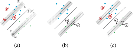
The analysis on complementary slackness conditions, i.e., Eqn. (2)-(3), leads to the partition of data into three sets:
which are shown in Figure 1(a), respectively. Besides, let αi = ζi - βi and S = L ∪ R is the index set of instances whose αi ̸= 0, the decision function can be rewritten as
3 ID-ODM for Single Instance Varying
In this section, we investigate the case when single instance comes or leaves.
3.1 Incremental Case
Suppose the new instance is (xk, yk). If γk ∈ [1 - θ, 1 + θ], acccording to Eqn. (4), this instance can be directly added to C without any update. Thus without loss of generality, we assume γk ̸∈ [1 - θ, 1 + θ] and initialize the Lagrange multiplier αk as 0. Next, we first derive the relationship between αS and αk, and then detail how to update αS by varying αk gradually.
The relationship between αS and αk. Notice that 1 ± θ are constants, to make the KKT conditions hold, i.e.,
the Lagrange multiplier αS should vary with αk such that
where ∆ denotes the variations of variables. With Eqn. (4), we have
Notice that αi = λξi for ∀i ∈ L and αi = -λϵi for ∀i ∈ R, we can derive the following linear system
where hij = yiyjκij . Denote H = (hij)i,j∈[k], then Eqn. (8) can be rewritten in a matrix form
which implies that ∆αS varies linearly with ∆αk:
Update αk. By substituting Eqn. (9) into Eqn. (7) to eliminate ∆αS , the remaining variable is only ∆αk. We can monitor the variation of margin with ∆αk for all instances.
Different from previous works like [Cauwenberghs and Poggio, 2000] in which αk belongs to [0, C] and can be simply updated by increasing gradually from 0 to C, here αk ∈ R is unbounded, and we do not even know whether to increase or decrease αk. Fortunately, if (xk, yk) is successfully added, by KKT conditions, we have
where
With Eqn. (7) and Eqn. (9), we have a closed-form solution
The above analysis is based on the assumption that the three index sets L, C, and R remain unchanged when αk is varying, thus Eqn. (12) is not an actual optimal solution, but it can provide a credible update direction. In practice, we can let ∆αk = η∆α⋆k and increases η from 0 to 1 gradually. At the same time, we monitor the three index sets. When one of the following events occurs
- i ∈ S migrates to C, i.e., nonzero αi turns to 0,
- i ∈ C migrates to S, i.e., f(xi) reaches the boundary of the strip as shown in Figure 1,
we call a breakpoint is detected and sequentially perform the following four steps
- Stop the increase of η.
- Update the index sets L, C, and R.
- Record the current αk and αS.
- Update H, t, and ∆α⋆k .
The above procedure is repeated until no breakpoint is detected during the increase of η from 0 to 1, then (xk, yk) can be added to L or R based on current γk.
3.2 Decremental Case
Suppose the invalid instance is (xk, yk). If k ∈ C, i.e., αk = 0, it has no contribution to the model and can be removed directly. Thus without loss of generality, we assume k ∈ S. Now we need to turn αk to 0 to totally eliminate its effect on the model. Analogous to the incremental case, we first update S = S \ {k} and derive the relationship between αS and αk, and then show how to update αS by varying αk.
The relationship between αS and αk. Since we should make KKT conditions hold at any time, the deletion of αk from S can be viewed as the reverse process of addition of αk to S. Again, ∆αS and ∆αk satisfy
Since ∆αS changes linearly with ∆αk, we can trace the variation of the margin with ∆αk.
Update αk. The update is now reduced to determine ∆αk. Distinct from the incremental case, the invalid data vanishes and the algorithm terminates with ∆α⋆k = -αk.
As a result, we can update αk with ∆αk = -ηαk. Like the incremental case, each update is comprised of four steps when we keep watch on breakpoints. The whole procedure stops when η = 1.
4 ID-ODM
In this section, we first present the general ID-ODM for multiple instances varying and then analyze the time complexity and convergence.
4.1 Multiple Instances Varying
Without loss of generality, we assume that there are p instances {(xi, yi)}i∈E becoming available and q instances {(xj, yj)}j∈I turning invalid where
We denote A = E ∪I to represent all varying instances for convenience. The most straightforward way is to view each single instance individually and invoke the method in Section 3.1 and 3.2 for p times and q times, respectively. Nevertheless, this scheme is computationally inefficient as shown in Figure 2(a).
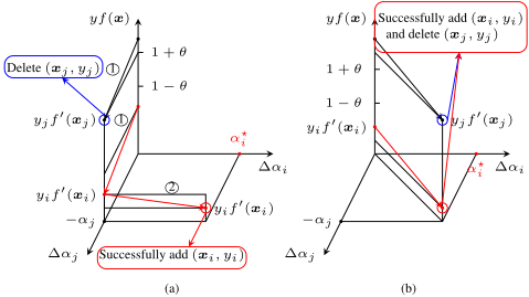
One smarter way is to update αE and αI simultaneously as shown in Figure 2(b). Under this circumstance, multiple new instances satisfy the optimal conditions, and multiple invalid instances are removed at the same time. In the same manner as before, we first update S = S \ I and derive the relationship between αS and αA, and then show how to update αE and αI simultaneously.
The relationship between αS and αA. Different from the single instance case where ∆αk is a scalar, now ∆αS varies with the vector ∆αA. The margin change of (xi, yi) is de-
In order to make KKT conditions hold, ∆αS, ∆αE, and ∆αI should satisfy
Thus, ∆αS can be traced by ∆αE and ∆αI according to
Update αA. The critical point to update the model lies in identifying ∆αA. Intuitively, αI is supposed to update along the opposite direction of αI to remove the invalid data. In other words, ∆αI = -ηαI. As for αE, we determine the update direction ∆αE by keeping KKT conditions w.r.t the new instances. Since multiple instances arrive, Eqn. (10) can be recast in
dE = γE + HES∆α⋆S + HEA∆α⋆A + (αE + ∆α⋆E )/λ, where d is the vector with the k-th entry dk defined in Eqn. (11). By denoting ∆αS via ∆αE and ∆αI, we can determine ∆α⋆E by
It seems that ∆α⋆E is relevant to ∆α⋆I , but when no breakpoint is produced, ∆α⋆I = -αI is fixed. Consequently, we update αA via
and track ∆αS and ∆f(x) by searching for the minimal η which will lead to a breakpoint or the termination of IDODM. Algorithm 1 summarizes the pseudo-code for IDODM.
4.2 Time Complexity
According to the Algorithm 1, the main time cost is caused by computing the inverse of the matrix QS. It is well accepted that the time complexity of computing the inverse of a n-order square matrix is O(n3 ). If we calculate Q-1 S at each iteration, the time complexity is O(c(m+p-q)3 ), where c is the number of breakpoints. Hence it is very time-consuming. However, by resorting to Sherman-Morrison-Woodbury formula [Golub and Van Loan, 1983], we can reduce the time cost to O(c(m+p- q)2 ).
Suppose a new instance (xc, yc) is added to S, let S ′ = S ∪ {c}, then we have
The Schur's complement [Zhang, 2006] of QS is S = κcc + 1/λ - HcSQ-1 S HSc. According to the Sherman-MorrisonWoodbury formula,
where v = -Q-1 S HSc.
As for the decremental case, we can exchange the roles of S and S ′ , and calculate Q-1 S ′ in the same manner.
Algorithm 1 ID-ODM
- 1: Input: The data set {(xi, yi)}i∈[m], the hyperparameters {λ, θ, σ}, the given model αS, the varying instances
{(xi, yi)}i∈E∪I . 2: Calculate the margin γ, and the matrix Q-1 , H, T. 3: for k ∈ E do 4: if γk ∈ [1- θ, 1+ θ] then 5: C = C ∪ {k}, E = E \ {k}. 6: end if 7: end for 8: for k ∈ I do 9: if k ∈ C then 10: C = C \ {k}, I = I \ {k}. 11: end if 12: end for 13: S = S \ I. 14: while true do 15: Calculate the update direction ∆αA. 16: Calculate the minimal η leading to breakpoints. 17: if η < 1 then 18: Update the index sets S and C. 19: Update Q-1 S , T, γ, αS and αA. 20: else 21: Break. 22: end if 23: end while 24: Output: The updated model αS.4.3 Convergence
According to Eqn. (9), ID-ODM depends on the existence of Q-1 S . Fortunately, for quadratic-type loss, Q is strictly diagonally dominant and positive definite, thus its inverse always exists.
When an instance (xk, yk) comes or leaves, αk varies, the classification hyperplane evolves, and αS monotonically increases or decreases [Laskov et al., 2006]. To guarantee the convergence of Algorithm 1, we should further prove the monotonic update of αS is strict, that is no instance migrates between index sets back and forth.
Theorem 1 (Immediate cycling will not occur). If a breakpoint (xc, yc) migrates from C to S or vice versa in round t, it will not come back in the next round.
Proof. C → S: Suppose (xc, yc) migrates from C to L. Before it enters L, we always have α(t) c = 0. If it comes back from L to C in the next round, its margin will increase, i.e., ∆γ (t+1) c > 0. Notice that ∆γi = -∆αi/λ, ∀i ∈ L according to Eqn. (5), which implies ∆α(t+1) c < 0. Together with α(t) c = 0, we have α(t+1) c < 0. A contradiction occurs since αi > 0, ∀i ∈ L.
The proof of migration from C to R is similar. If (xc, yc) comes back from R to C in the next round, its margin will decrease, and we have ∆γ (t+1) c < 0 and ∆α(t+1) c > 0 by noticing that ∆γi = -∆αi/λ, ∀i ∈ R according to Eqn. (6). Together with α(t) c = 0, we have α(t+1) c > 0, which contradicts with αi < 0, ∀i ∈ R.
S → C: It is equivalent to prove that the margin varies monotonically, i.e., ∆γ (t+1) c and ∆γ (t) c have the same sign.
Before a breakpoint turns out in round t, the index sets are S (t-1) and C (t-1) . Obviously the migration of (xc, yc) from S (t-1) to C (t) can be viewed as the reverse process of migration from C (t) to S (t-1) . Thus, we can calculate t(t) as
where S is the Shur's complement of QS (t-1) , and the first and last equality are according to the definition of t, v, and Eqn. (15), respectively. With Eqn. (16), we have
Then we can further calculate the variation of margin for the instance (xc, yc) in round t + 1 as
where the first and third equality are according to Eqn. (7) and Eqn. (9), respectively. With Eqn. (17), we have ∆γ (t+1) c = -S∆α(t) c ∆α(t+1) k /∆α(t) k .
Since the update of αk is monotonic, ∆α(t) k and ∆α(t+1) k have the same sign. Notice that ∆α(t) c has the opposite sign to ∆γ (t) c , thus ∆γ (t+1) c has the same sign with ∆γ (t) c if S > 0. Since QS is a positive definite matrix, the corresponding Shur's complement S > 0 [Ouellette, 1981], which concludes the proof. For multiple instance changes, the proof is similar.
5 Experiments
In this section, we empirically analyze the effectiveness and efficiency of our proposed methods.
5.1 Setup
Data sets. We perform experiments on nine real-world data sets available on the LIBSVMwebsite 1 . The features of each data set are normalized into [0, 1]. The characteristics of data sets are summarized in Table 2. We randomly divide all data sets into training and test sets with a ratio of 4:1. Besides, we randomly select 75% of the training data as historical data and the rest are varying data.
1 https://www.csie.ntu.edu.tw/∼cjlin/libsvmtools/datasets/binary. html
| ID | Data sets | #Instances | #Features |
|---|---|---|---|
| 1 | heart | 270 | 13 |
| 2 | ionosphere | 351 | 34 |
| 3 | breast | 683 | 10 |
| 4 | diabetes | 768 | 8 |
| 5 | fourclass | 862 | 2 |
| 6 | splice | 1,000 | 60 |
| 7 | svmguide3 | 1,243 | 21 |
| 8 | madelon | 2,000 | 500 |
| 9 | a2a | 2,265 | 123 |
Methods. To make an overall comparison, we implement single incremental and decremental ODM (SID-ODM) and batch incremental and decremental ODM (BID-ODM). We use historical data to train the initial ODM and all varying instances will be added to the model and then deleted. SIDODM adds/deletes an instance at once while BID-ODM processes a batch of data. The batch size is set to 5. Apart from our proposed methods, we retrain the model for comparison, which is denoted as SR-ODM and BR-ODM corresponding to single and multiple varying instances, respectively. All methods are performed on a machine with the 11th Gen Intel(R) Core(TM) i5-11320H@3.20GHz CPUs and 16GB main memory. ODM is optimized by dual coordinate gradient descent.
Hyperparameters. The hyperparameters in our experiments contain three model hyperparameters {λ, θ, σ}. λ and θ are tuned from {10-3 , . . . , 103 } and {0.1, 0.2, . . . , 0.9}, respectively by grid search. The kernel hyperparameter σ is fixed to 1/d where d is the number of features. All experiments are performed five times according to different data partitions.
Evaluation Measures. To verify the efficiency of our proposed methods, we compare the running time of each method. Besides, we also compare the accuracy on the test set to validate the effectiveness. We record the average accuracy as well as the standard deviation.
| Data sets | Time (in seconds) | Speedup Ratio | |||||
|---|---|---|---|---|---|---|---|
| SR-ODM | SID-ODM | BR-ODM | BID-ODM | SID/SR | BID/BR | BID/SID | |
| heart ionosphere breast diabetes fourclass splice svmguide3 madelon a2a | 0.007±0.001 0.012±0.002 0.033±0.005 0.040±0.006 0.047±0.007 0.197±0.031 0.127±0.020 3.001±0.470 0.443±0.071 | 0.001±0.001 0.001±0.001 0.004±0.003 0.008±0.004 0.009±0.004 0.022±0.015 0.024±0.012 0.078±0.079 0.082±0.054 | 0.007±0.003 0.011±0.002 0.033±0.005 0.041±0.006 0.047±0.007 0.198±0.030 3.116±0.496 | 0.001±0.001 0.002±0.001 0.006±0.004 0.007±0.002 0.009±0.005 0.037±0.018 0.024±0.018 0.132±0.080 0.102±0.055 | 11.68 10.57 7.50 5.32 5.42 8.85 5.31 38.41 5.42 | 5.55 5.59 5.50 5.66 5.33 5.43 5.31 23.56 4.29 | 2.16 2.78 3.61 5.21 4.88 3.05 4.95 2.95 4.00 |
| 0.128±0.020 | |||||||
| 0.438±0.066 | |||||||
5.2 Results
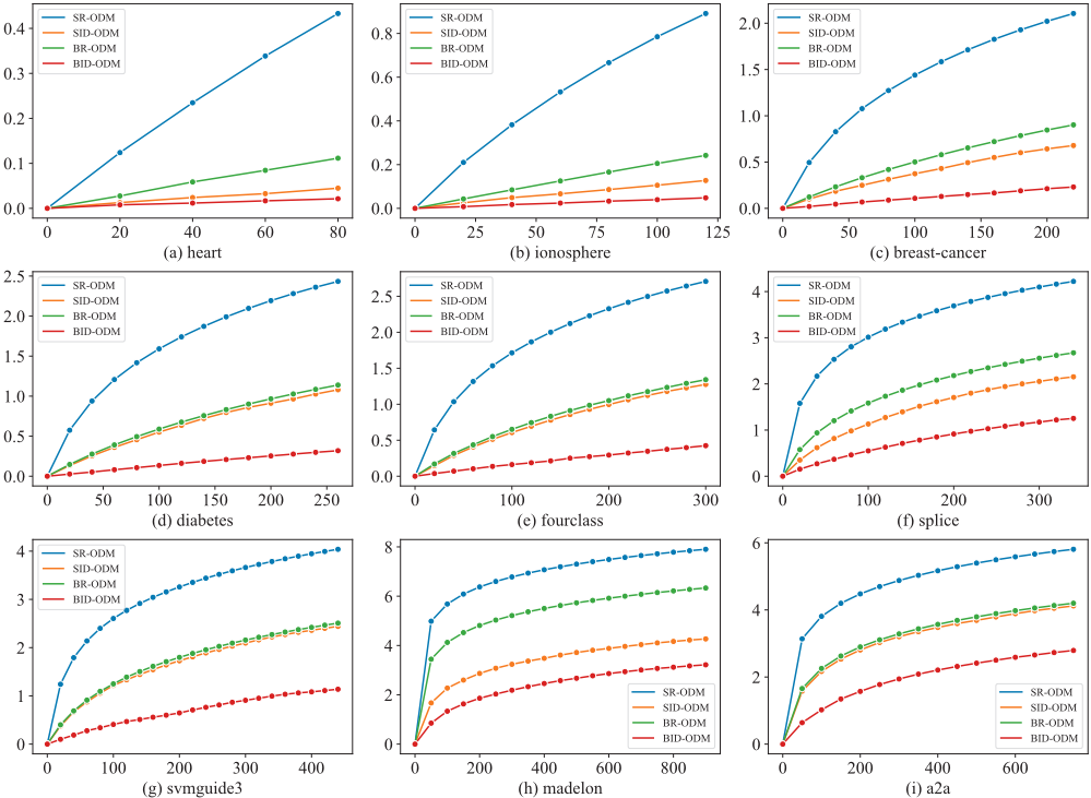
Efficiency Comparison. Figure 3 demonstrates the cumulative running time of conducting SID-ODM, BID-ODM, SR-ODM, and BR-ODM on each data set. It can be seen that both SID-ODM and BID-ODM cost much less time than retraining the model from scratch, which reveals the efficiency of our proposed method. Besides, it is worth noting that the running time of SR-ODM and BR-ODM varies significantly with the data size while SID-ODM and BID-ODM behave steadily, which benefits from the Sherman-MorrisonWoodbury formula.
Table 3 further shows the speedup ratio of our proposed methods compared to retraining the model. Since data sets have various characteristics, the boost of the performance differs slightly, but on all data sets, we can gain more than 4 times acceleration and even can reach 9.1× speedup on average. Besides, there is no doubt that BID-ODM is more efficient than SID-ODM since it processes multiple instances at one time but with a closed-time cost to SID-ODM. The speedup ratio of BID-ODM compared to SID-ODM is also recorded in Table 3 to make an intuitive comparison.
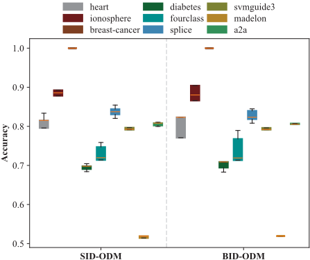
Generalization Performance Comparison. Figure 4 shows the accuracy over 5 trials with a box plot. We also plot the mean accuracy of retraining the model in the box. Intuitively, our proposed methods accelerate the update of ODM nearly without sacrificing accuracy, which validates the effectiveness of our proposed methods.
In order to further validate the performance of ID-ODM, we compare it with MID-SVM [Karasuyama and Takeuchi, 2009], which is another batch IDL method based on SVM. We incrementally add 100 instances to the training set and record the accuracy. As shown in Table 4, ID-ODM performs better than MID-SVM on most datasets, which benefits from optimizing margin distribution.
| Data sets | ID-ODM | MID-SVM |
|---|---|---|
| heart ionosphere breast diabetes fourclass splice svmguide3 madelon a2a | 81.5 ± 4.7 87.4± 6.6 97.2 ± 0.9 76.9 ± 4.8 78.7 ± 2.8 84.4 ± 3.1 80.5 ± 1.5 58.0 ± 1.1 | 81.1 ± 4.1 90.6 ± 3.8 96.7 ± 1.2 76.6 ± 4.9 77.1 ± 1.9 85.5 ± 3.6 79.9 ± 1.3 56.7 ± 1.6 |
| Avg. Acc. | 81.1 | 80.8 |
| 83.0 ± 0.8 | 83.0 ± 0.8 |
6 Conclusions
In this paper, we propose the ID-ODM to efficiently update ODM when new data is available or old data turns invalid. Specifically, we avoid updating the unbounded Lagrange multipliers in an infinite range by estimating the optimal value beforehand, thus iteratively updating the model. Moreover, ID-ODM is effective no matter how data varies, thus it is applicable to various real-world tasks. Besides, we provide some theoretical analysis on ID-ODM. Extensive experiments validate the effectiveness and efficiency of our method. In the future, we will extend our method to other models with quadratic-type loss.
Acknowledgments
This work was supported in part by the National Key R&D Program of China under Grant 2020AAA0108501, the National Natural Science Foundation of China under Grant 62006088, and the Key R&D Program of Hubei under Grant 2020BAA020.
@inproceedings{ijcai2023p392,
  title     = {Incremental and Decremental Optimal Margin Distribution Learning},
  author    = {Chen, Li-Jun and Zhang, Teng and Shi, Xuanhua and Jin, Hai},
  booktitle = {Proceedings of the Thirty-Second International Joint Conference on
               Artificial Intelligence, {IJCAI-23}},
  publisher = {International Joint Conferences on Artificial Intelligence Organization},
  editor    = {Edith Elkind},
  pages     = {3523--3531},
  year      = {2023},
  month     = {8},
  note      = {Main Track},
  doi       = {10.24963/ijcai.2023/392},
  url       = {https://doi.org/10.24963/ijcai.2023/392},
}
TY - CPAPER TI - Incremental and Decremental Optimal Margin Distribution Learning AU - Chen, Li-Jun AU - Zhang, Teng AU - Shi, Xuanhua AU - Jin, Hai T2 - Proceedings of the Thirty-Second International Joint Conference on Artificial Intelligence, IJCAI-23 PB - International Joint Conferences on Artificial Intelligence Organization PY - 2023 SP - 3523 EP - 3531 DO - 10.24963/ijcai.2023/392 UR - https://doi.org/10.24963/ijcai.2023/392 ER -Copied
Machine-readable versions of this paper, for tools and AI agents:





