
Some General Identification Results for Linear Latent Hierarchical Causal Structure
Proceedings of the Thirty-Second International Joint Conference on Artificial Intelligence. Main Track. Pages 3568-3576.
https://doi.org/10.24963/ijcai.2023/397
Keywords
- Uncertainty in AI: UAI: Causality, structural causal models and causal inference
- Machine Learning: ML: Causality
Abstract
We study the problem of learning hierarchical causal structure among latent variables from measured variables. While some existing methods are able to recover the latent hierarchical causal structure, they mostly suffer from restricted assumptions, including the tree-structured graph constraint, no ``triangle" structure, and non-Gaussian assumptions. In this paper, we relax these restrictions above and consider a more general and challenging scenario where the beyond tree-structured graph, the ``triangle" structure, and the arbitrary noise distribution are allowed. We investigate the identifiability of the latent hierarchical causal structure and show that by using second-order statistics, the latent hierarchical structure can be identified up to the Markov equivalence classes over latent variables. Moreover, some directions in the Markov equivalence classes of latent variables can be further identified using partially non-Gaussian data. Based on the theoretical results above, we design an effective algorithm for learning the latent hierarchical causal structure. The experimental results on synthetic data verify the effectiveness of the proposed method.
- [Adams et al., 2021] J. Adams, N. Hansen, and K. Zhang. Identification of partially observed linear causal models: Graphical conditions for the non-gaussian and heteroge- neous cases. In Advances in Neural Information Process- ing Systems, 2021.
- [Anandkumar et al., 2013] Animashree Anandkumar, Daniel Hsu, Adel Javanmard, and Sham Kakade. Learn- ing linear bayesian networks with latent variables. In International Conference on Machine Learning, pages 249-257, 2013.
- [Bartholomew et al., 2008] David Bartholomew, Fiona Steele, Ir Moustaki, and Jane Galbraith. The analysis and interpretation of multivariate data for social scientists. Routledge (2 edition), 2008.
- [Bollen, 1989] Kenneth A. Bollen. Structural Equations with Latent Variable. John Wiley & Sons, 1989.
- [Cai et al., 2019] Ruichu Cai, Feng Xie, Clark Glymour, Zhifeng Hao, and Kun Zhang. Triad constraints for learn- ing causal structure of latent variables. In NeurIPS, pages 12863-12872, 2019.
- [Chen et al., 2022] Zhengming Chen, Feng Xie, Jie Qiao, Zhifeng Hao, Kun Zhang, and Ruichu Cai. Identification of linear latent variable model with arbitrary distribution. In Proceedings 36th AAAI Conference on Artificial Intelli- gence (AAAI), 2022.
- [Chickering, 2002] David Maxwell Chickering. Optimal structure identification with greedy search. JMLR, 3(Nov):507-554, 2002.
- [Choi et al., 2011a] Myung Jin Choi, Vincent Y.F. Tan, Ani- mashree Anandkumar, and Alan S. Willsky. Learning la- tent tree graphical models. Journal of Machine Learning Research, 12(49):1771-1812, 2011.
- [Choi et al., 2011b] Myung Jin Choi, Vincent YF Tan, Ani- mashree Anandkumar, and Alan S Willsky. Learning la- tent tree graphical models. Journal of Machine Learning Research, 12:1771-1812, 2011.
- [Colombo et al., 2012] Diego Colombo, Marloes H Maathuis, Markus Kalisch, and Thomas S Richard- son. Learning high-dimensional directed acyclic graphs with latent and selection variables. The Annals of Statistics, pages 294-321, 2012.
- [Cui et al., 2018] Ruifei Cui, Perry Groot, Moritz Schauer, and Tom Heskes. Learning the causal structure of cop- ula models with latent variables. In Proceedings of the Thirty-Fourth Conference on Uncertainty in Artificial In- telligence, UAI 2018, pages 188-197. AUAI Press, 2018.
- [Drton et al., 2017] Mathias Drton, Shaowei Lin, Luca Weihs, and Piotr Zwiernik. Marginal likelihood and model selection for gaussian latent tree and forest models. Bernoulli, 23(2):1202-1232, 2017.
- [Hoyer et al., 2009] Patrik O Hoyer, Dominik Janzing, Joris M Mooij, Jonas Peters, and Bernhard Schölkopf. Nonlinear causal discovery with additive noise models. In NeurIPS, pages 689-696, 2009.
- [Huang et al., 2022] Biwei Huang, Charles Jia Han Low, Feng Xie, Clark Glymour, and Kun Zhang. Latent hier- archical causal structure discovery with rank constraints. In Advances in Neural Information Processing Systems, 2022.
- [Kitson et al., 2021] Neville K Kitson, Anthony C Con- stantinou, Zhigao Guo, Yang Liu, and Kiattikun Chobtham. A survey of bayesian network structure learn- ing. arXiv preprint arXiv:2109.11415, 2021.
- [Kivva et al., 2021] Bohdan Kivva, Goutham Rajendran, Pradeep Ravikumar, and Bryon Aragam. Learning latent causal graphs via mixture oracles. Advances in Neural In- formation Processing Systems, 34, 2021.
- [Kummerfeld and Ramsey, 2016] Erich Kummerfeld and Joseph Ramsey. Causal clustering for 1-factor mea- surement models. In KDD, pages 1655-1664. ACM, 2016.
- [Kummerfeld et al., 2014] Erich Kummerfeld, Joe Ramsey, Renjie Yang, Peter Spirtes, and Richard Scheines. Causal clustering for 2-factor measurement models. In Pro- ceedings of the 2014th European Conference on Machine Learning and Knowledge Discovery in Databases-Volume Part II, pages 34-49, 2014.
- [Mourad et al., 2013] Raphaël Mourad, Christine Sinoquet, Nevin L Zhang, Tengfei Liu, and Philippe Leray. A survey on latent tree models and applications. Journal of Artificial Intelligence Research, 47(1):157-203, 2013.
- [Pearl, 1988a] Judea Pearl. Probabilistic Reasoning in In- telligent Systems: Networks of Plausible Inference. Mor- gan Kaufmann Publishers Inc., San Francisco, CA, USA, 1988.
- [Pearl, 1988b] Judea Pearl. Probabilistic Reasoning in In- telligent Systems: Networks of Plausible Inference. Mor- gan Kaufmann Publishers Inc., San Francisco, CA, USA, 1988.
- [Pearl, 2009] Judea Pearl. Causality: Models, Reasoning, and Inference. Cambridge University Press, New York, 2nd edition, 2009.
- [Peters et al., 2017] Jonas Peters, Dominik Janzing, and Bernhard Schölkopf. Elements of Causal Inference. MIT Press, 2017.
- [Poon et al., 2010] Leonard KM Poon, Nevin L Zhang, Tao Chen, and Yi Wang. Variable selection in model-based clustering: to do or to facilitate. In Proceedings of the 27th International Conference on International Conference on Machine Learning, pages 887-894, 2010.
- [Shafera et al., 1993] Glenn Shafera, Alexander Koganb, and Peter Spirtesc. Generalization of the tetrad represen- tation theorem. DIMACS Technical Report 93-68, 1993.
- [Shimizu et al., 2006] Shohei Shimizu, Patrik O Hoyer, Aapo Hyvärinen, and Antti Kerminen. A linear non- Gaussian acyclic model for causal discovery. JMLR, 7(Oct):2003-2030, 2006.
- [Shimizu et al., 2009] Shohei Shimizu, Patrik O Hoyer, and Aapo Hyvärinen. Estimation of linear non-gaussian acyclic models for latent factors. Neurocomputing, 72(7- 9):2024-2027, 2009.
- [Silva et al., 2006] Ricardo Silva, Richard Scheine, Clark Glymour, and Peter Spirtes. Learning the structure of lin- ear latent variable models. JMLR, 7(Feb):191-246, 2006.
- [Spearman, 1928] Charles Spearman. Pearson's contribution to the theory of two factors. Br. J. Psychol., 19(1):95-101, 1928.
- [Spirtes and Glymour, 1991] Peter Spirtes and Clark Gly- mour. An algorithm for fast recovery of sparse causal graphs. Social science computer review, 9(1):62-72, 1991.
- [Spirtes and Zhang, 2016] Peter Spirtes and Kun Zhang. Causal discovery and inference: concepts and recent methodological advances. In Applied informatics, vol- ume 3, pages 1-28. SpringerOpen, 2016.
- [Spirtes et al., 1995] Peter Spirtes, Christopher Meek, and Thomas Richardson. Causal inference in the presence of latent variables and selection bias. In UAI, pages 499-506.
- [Spirtes et al., 2000] Peter Spirtes, Clark Glymour, and Richard Scheines. Causation, Prediction, and Search. MIT press, 2000.
- [Squires et al., 2022] C. Squires, A. Yun, E. Nichani, R. Agrawal, and C. Uhler. Causal structure discovery between clusters of nodes induced by latent factors. In CLeaR, 2022.
- [Xie et al., 2020] Feng Xie, Ruichu Cai, Biwei Huang, Clark Glymour, Zhifeng Hao, and Kun Zhang. Generalized independent noise conditionfor estimating latent variable causal graphs. In NeurIPS, pages 14891-14902, 2020.
- [Xie et al., 2022] Feng Xie, Biwei Huang, Zhengming Chen, Yangbo He, Zhi Geng, and Kun Zhang. Identification of linear non-gaussian latent hierarchical structure. In Inter- national Conference on Machine Learning, pages 24370- 24387. PMLR, 2022.
- [Xie et al., 2023] Feng Xie, Yan Zeng, Zhengming Chen, Yangbo He, Zhi Geng, and Kun Zhang. Causal discovery of 1-factor measurement models in linear latent variable models with arbitrary noise distributions. Neurocomput- ing, 2023.
- [Zeng et al., 2021] Yan Zeng, Shohei Shimizu, Ruichu Cai, Feng Xie, Michio Yamamoto, and Zhifeng Hao. Causal discovery with multi-domain lingam for latent factors. In IJCAI, pages 2097-2103, 2021. IJCAI
- [Zhang and Hyvärinen, 2009] Kun Zhang and Aapo Hyvärinen. On the identifiability of the post-nonlinear causal model. In UAI, pages 647-655. AUAI Press, 2009.
- [Zhang, 2004] Nevin L Zhang. Hierarchical latent class models for cluster analysis. The Journal of Machine Learning Research, 5:697-723, 2004.
- [Zhang, 2008] Jiji Zhang. On the completeness of orienta- tion rules for causal discovery in the presence of latent confounders and selection bias. Artificial Intelligence, 172(16-17):1873-1896, 2008.
- [Zhou et al., 2020] Can Zhou, Xiaofei Wang, and Jianhua Guo. Learning mixed latent tree models. Journal of Ma- chine Learning Research, 21(249):1-35, 2020.
References were extracted automatically from the PDF and may contain errors.
Full text extracted automatically from the PDF; figures, tables and equations may differ. The PDF is the version of record.
1 Introduction
In the traditional causal discovery task, researchers focus on discovering the causal relationships between the measured (observed) variables [Pearl, 2009; Spirtes et al., 2000; Peters et al., 2017]. There have been a number of attempts to address this issue [Spirtes and Glymour, 1991; Chickering, 2002; Shimizu et al., 2006; Hoyer et al., 2009; Zhang and Hyv¨arinen, 2009; Spirtes et al., 1995; Zhang, 2008; Colombo et al., 2012] (also see [Spirtes and Zhang, 2016; Kitson et al., 2021]). However, in some empirical studies, scientists are interested in inferring causal relationships between latent (hidden) variables that they cannot directly measure, e.g., the relationship between industrialization and political democracy [Bollen, 1989; Bartholomew et al., 2008].
∗Corresponding author.
Thus, it is necessary to develop statistical methods for learning the causal relationships between latent variables.
By the measured variables that are influenced by the latent variables, much effort has been made to recover causal structure among latent variables, such as Tetrad constraint-based methods [Silva et al., 2006; Kummerfeld et al., 2014; Kummerfeld and Ramsey, 2016; Xie et al., 2023], non-Gaussianity based-approaches [Shimizu et al., 2009; Cai et al., 2019; Xie et al., 2020; Zeng et al., 2021; Adams et al., 2021; Chen et al., 2022], expansion property-based method [Anandkumar et al., 2013], copula model-based method [Cui et al., 2018], and mixture oracle-based method [Kivva et al., 2021]. However, these methods assume that each latent variable has some certain measured variables as children and fail to work when latent variables have no measured variables.
There exist several works in the literature that tried to recover the latent hierarchical causal structure (i.e., the children of some latent variables may still be latent variables). One classical framework for inferring latent hierarchical structure is the latent tree model [Pearl, 1988a; Zhang, 2004]. Many contributions along this line include [Poon et al., 2010; Choi et al., 2011a; Mourad et al., 2013; Drton et al., 2017; Zhou et al., 2020]. However, these methods assume that the underlying structure is a tree-structured graph (there is only one path between every pair of variables in the graph). In realworld scenarios, they may not be tree-structured graphs. Recently, [Xie et al., 2022] relaxed the tree-structured assumption and provided a sufficient graphical condition for identifying the latent hierarchical causal structure in the Linear NonGaussian Latent Hierarchical Model (LiNGLaM). They proposed a principled method to learn the latent causal structure by using the non-Gaussianity of noise variables. However, this method is inapplicable to partially Gaussian data. More recently, [Huang et al., 2022] relax the non-Gaussianity assumption and provided a new sufficient condition for recovering the structure in the linear latent hierarchical structure. They proposed a rank-deficiency constraint-based method to search the latent hierarchical structure. Though the proposed method does not restrict the non-Gaussinaity assumption, it assumes that there is no "triangle" structure, i.e., the child of the latent variable must be pure (without other parents), and cannot distinguish between Markov equivalent models over latent variables. Moreover, if the data is partially Gaussian, e.g., the setting described in Fig. 1, the above two methods will give incorrect or uninformative answers.
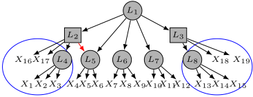
We seek to find out new general identifiability conditions of linear latent hierarchical causal structure in the case where the structure is not limited to a tree-structured graph without "triangle", and moreover, the data can be partially Gaussian. Meanwhile, we develop an efficient algorithm with theoretical guarantees to answer the following questions. (1) How can we locate the latent variables and recover the causal skeleton between them only from measured variables? (2) How can we infer the causal direction among latent variables by capturing the partially non-Gaussianity? Interestingly, these questions can be well addressed under appropriate conditions, by combining the Tetrad conditions and Generalized Independent Noise (GIN) conditions in specific ways.
Our contributions are summarised as follows:
- We develop new sufficient identifiability conditions that relax the existing assumptions, e.g., no "triangle" structure, and non-Gaussian assumption.
- We design an algorithm that can efficiently locate latent variables and identify the latent hierarchical structure up to a Markov equivalent class by leveraging Tetrad constraints, and meanwhile, can infer the causal direction in the causal skeleton by testing GIN conditions.
- We theoretically show that the proposed algorithm can find the correct hierarchical structure asymptotically under mild conditions.
2 Problem Statement
2.1 Linear Latent Hierarchical Model
In this paper, we focus on a linear latent hierarchical causal model with graph G, where both measured (observed) variables XG and latent variable LG are generated by their latent parents in a directed acyclic graph (DAG) with the following linear structural equation models:
where βij and αjk represent the causal strength from Lj to Xi and from Lk to Lj, respectively, and εXi and εLj are noise terms that are independent of each other. Without loss of generality, we assume that all variables in XG and LG have zero mean. Furthermore, Let VG denote all variables in a graph G, V, X and L be a set of variables, set of measured variable and a set of latent variables, respectively. We use Pa(Vi) = {Vj∣Vj → Vi}, Ch(Vi) = {Vj∣Vi → Vj}, Anc(Vi) = {Vj∣Vj ↝ Vi}, Des(Vi) = {Vj∣Vi ↝ Vj} to denote the set of parents, children, ancestors, descendants of Vi, respectively.
Definition 1 (Linear Latent Hierarchical Model (LHM)). A graphical model, with its graph G = (VG,EG), is a linear latent hierarchical model if:
- VG = XG ∪LG, where XG is the set of measured variables and LG is the set of latent variables,
- there is at least one undirected path between every pair of variables, and
- each variable inXG and LG are generated by the structural equation models in Eq. 1.
Goal. In this paper, we aim to establish newgeneral sufficient conditions of the latent hierarchical causal structure and also design an efficient algorithm for learning the latent hierarchical causal structure only from measured variables XG.
2.2 General Identifiability Conditions for LHM
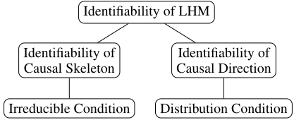
It is worth noting that, without further assumptions, there is no hope to locate latent variables in an LHM. Recent evidence suggests that under certain assumptions, e.g., tree-structured graph assumption [Pearl, 1988b; Zhang, 2004; Choi et al., 2011b], no "triangle" structure assumption [Huang et al., 2022], or non-Gaussian model assumption [Xie et al., 2022], the latent hierarchical structure is identifiable. However, these assumptions are restrictive and may not hold in practice, e.g., for the example given in Figure 1. Below, we describe sufficient general conditions under which the LHM becomes identifiable. Specifically, the task of identifiability of LHM can be divided into two sub-problem: identifiability of causal skeleton under Irreducible condition, and identifiability of causal direction under Distribution condition, as shown in Fig. 2.
Before giving the details of these two identifiability conditions, we first introduce a concept, Children sets, which will be used in the identifiability condition.
Definition 2 (Children Set). A variable set, denote by Vchild, is a children set of latent variable L in a graph G if Vchild ⊂ Ch(L).
We now give the condition for structural identifiability from measured variable XG .
Condition 1 (Irreducible Condition). The irreducible condition of linear latent hierarchical structure G satisfies:
- (1). for each latent variable Lp ∈ LG, there exists a children set Vchild of Lp with its partition Vchild = V1 ∪ V2 ∪V3 with ∣Vi∣ ≥ 1, such that (a) ∀Lq ∈ LG, Lq /∈ Des(Vchild), Vchild ⫫ {Lq} ∪ Des(Lq)∣Lp and (b) V1 ⫫ V2 ⫫ V3∣Lp,
- (2). there exists a neighbour set B to L s.t. B∩Vchild = ∅ and Dim(B) ≥ 1.
The key difference to existing researchers introducing the similar "irreducible condition", such as [Huang et al., 2022], is that we relax this assumption and allow the triangle structure (i.e., children of a latent variable may not be entirely pure). Fig. 1 shows a simple example that satisfies the proposed irreducible condition 1 whereas violates the "irreducible condition" given in [Huang et al., 2022] (the reason is that the children of L1, i.e., {L2,L5,L6,L7,L3}, are not fully pure due to the edge L2 → L5.).
The irreducible condition only ensures structural identifiability up to a Markov equivalent class, i.e., there are some edges that are undirected (see the Theorem 2). To further identify the causal direction of the undirected edge in the Markov equivalent class, the non-Gaussinaity of noise terms has been shown to be needed [Shimizu et al., 2006; Cai et al., 2019]. However, those works need to assume that all noise terms are non-Gaussian distributions. Interestingly, we found that the non-Gaussianity assumption can be relaxed to only a (hopefully small) subset of variables that are nonGaussian (see the Theorem 3). We refer to the Distribution condition in Condition 2.
Condition 2 (Distribution Condition). For each pair of adjacent latent variables Li, Lj in the causal skeleton G ′ , (1) at least one of latent variables Li, Lj has non-Gaussian noise or (2) there exists a latent variable Lk ∈ {Anc(Li)∪Anc(Lj)} that has non-Gaussian component ε such that ε is not conditional independent from {Li,Lj} given the confounder set S = {Pa(Li) ∩Pa(Lj)}, i.e., ε /⫫ (Li,Lj)∣S.
Compared to existing work introducing the nonGaussianity assumption, such as [Xie et al., 2022], Condition 2 allows for identifying the causal direction in the more general non-Gaussian setting. For example, as shown in Fig. 1, the triangle structure among L1,L2, and L5 are identifiable even if there is only L2 has non-Gaussian noise.
3 Algorithm for Estimating LHM
In this section, we propose a two-step efficient algorithm (Algorithm 1) to discover the structure of the linear latent hierarchical structure from measured variables. The algorithm covers two aspects of the identifiability problem that are shown in Fig. 2. Specifically, it first discovers the causal skeleton of LHM up to a Markov equivalent class in a recursive manner (Step I), and then infers the causal direction among the latent variable in the Markov equivalent class (Step II). The complete procedure is summarized in Algorithm 1.
1 For the latent variable L1, (1) there is a children set Vchild = {L2,L5,L6,L7} with its partition {L2,L5}, {L6} and {L7}, and (2) there exist a neighbor set B = {L3} satisfies the above two conditions.
Algorithm 1 Causal Discovery in LHM
Input: Data from a set of measured variables XG
Output: Partial causal structure G1
- 1: Initialize the active variable set A≔XG, and G ′ = ∅;
- 2: // Step I: Identify Causal Skeleton
- 3: Begin the recursive procedure
- 4: C = FindCausalClusters(A);
// Step 1.1
- 5: L, G ′ = IntroduceLatentVariables(C, G ′ ); // Step 1.2
- 6: A, G ′ = UpdateCausalSkeleton(L, G ′ );
- // Step 1.3
- 7: End the recursive procedure Until no causal cluster is found or new latent variable is introduced
- 8: // Step II: Identify Causal Direction
- 9: G = OrientEdges(XG, G ′ );
- 10: return Graph G.
Below, we provide the technical details of the two steps.
3.1 Step I: Identify Causal Skeleton
We adopt a recursive procedure to identify the causal skeleton (Step 1.1 ∼ Step 1.3). More specifically, in Step 1.1, the causal cluster will be learned from the active variable set. In Step 1.2, according to the learned causal cluster, the new latent variable set will be introduced without redundancy. In Step 1.3, the causal skeleton is reconstructed from the output of the previous phase, and the active variable is updated such that the new causal cluster can be learned in the next iteration. By repeating the above phases until no new causal cluster is learned or no new latent variable is introduced, the skeleton will be recovered (Line 3 ∼ 7 in Algorithm 1).
Before giving the details of Step I, we first give a theorem that relates the latent hierarchical structure to the Tetrad constraints over measured variables.
Theorem 1 (Graphical Implication of Tetrad Constraint in LHM). Suppose G satisfies a linear latent hierarchical model and the irreducible condition holds. Then two measured variables set XA and XB in G (with Dim(XA),Dim(XB) ≥ 2) is d-separated by a latent variable in G if and only if ∀Xi,Xj ∈ XA, ∀Xk,Xs ∈ XB, {Xi,Xj} and {Xk,Xs} follows Tetrad Constraints, i.e., σXiXk σXjXs = σXiXs σXjXk , where σViVj is the co-variance between Vi and Vj and it is not equal to zero.
Example 1. Consider the structure in Fig. 1. Let X = {X7, X8, X9}. We can verify that ∀Xi, Xj ∈ X, ∀Xk, Xs ∈ XG \X, where XG = {X1, ..., X19}, {Xi, Xj} and {Xk, Xs} follows Tetrad Constraints. This is because L1 d-separates X from XG \ X.
The classical Tetrad constraint [Spearman, 1928; Shafera et al., 1993] has been used in the past to investigate linear latent variable models under pure measurement model assumption [Silva et al., 2006; Kummerfeld and Ramsey, 2016]. The current study extends the application scenario and utilizes Tetrad constraints to analyze the causal structure of the linear latent hierarchical model under some general conditions (beyond the pure measurement model).
Step 1.1: Find Causal Clusters
Step I begins with examining the existence of latent variables by identifying the causal clusters in the active variable set 2 . We denote the active variable set as A, which is set to XG initially. Next, we give the definition of the causal cluster and provide a method to identify the causal cluster from the active variable set (Proposition 1).
Definition 3 (Causal Cluster &Minimal Causal Cluster). Let A be the active variable set that is under investigation. We say a set C ⊂ A is a causal cluster if there exists a latent variable L such that L d-separates C from A\C. Furthermore, we say C is a minimal causal cluster if no proper subset ˜C ⊂ C (with Dim( ˜C) ≥ 2) is a causal cluster.
It is worth noting that for a minimal causal cluster C, if C is a pure child set of a latent variable L, then the dimension of C is two and ∀Vi, Vj ∈ C, Vi ⫫ Vj∣L. To distinguish the property of the causal clusters, we give a brief definition of the pure (impure) causal cluster, which will be used in the next phase. Generally, we use the pure (impure) causal cluster to refer to any pair variable of C that is (not) d-separated by a latent variable L, i.e., C is a pure causal cluster if there exists a latent variable L such that ∀Vi, Vj ∈ C, Vi ⫫ Vj∣L. For example, consider the structure in Fig. 1. Suppose the active variable set A = {L2, L5, L6, L7, L8}. C1 = {L6, L7} is a pure causal cluster while C2 = {L2, L5} is a impure causal cluster.
We next show that the minimal causal cluster, fortunately, will help us to find the existence of the latent variables, which can be identified by appropriately testing for the Tetrad constraint, as formally stated in the following proposition.
Proposition 1 (Identify Minimal Causal Cluster). Let A be the active variable set and C be a proper subset of A. Then C is a minimal causal cluster if and only if the following two conditions hold 1) ∀Vi, Vj ∈ C, ∀Vk, Vs ∈ A \ C, {Vi, Vj} and {Vk, Vs} follows Tetrad Constraints, and 2) no proper subset of C satisfies condition 1).
According to Proposition 1, given an active variable set, one may identify all minimal causal clusters in the current active variable set. The detailed search procedure of Step 1.1 is given in Algorithm 2 (named FindCausalClusters). Specifically, given an active variable set A, we first identify the causal cluster with size CLen = 2 based on Proposition 1 from all possible combinations. Then we increase the size of finding causal cluster Ci until no causal cluster of the active variable set is found. An illustrative example is given below.
Example 2. Consider the causal structure in Fig. 1. Suppose active variable set A = {X1, ...,X19}. Let the size of causal cluster CLen = 2, one can find seventeen clusters, i.e., {X1,X2}, {X1,X3}, {X2,X3} ..., {X18,X19} .
Step 1.2: Introduce Latent Variables
By Algorithm 2 (FindCausalClusters), we already find all minimal causal clusters in active set A. This will tell us that there exist latent variables for those minimal causal clusters. However, if we directly introduce the latent variable for the
2 We say a set is active if selected in the current iteration.
Algorithm 2 FindCausalClusters
Input: A set of active variables A Output: Causal Cluster set C
- 1: Let C = ∅ be a causal cluster set, and B is a copy of
active variable set A; 2: Initialize the finding causal size CLen = 2; 3: for ∣B∣ ≥ CLen + 2 do 4: for draw a set of test variables Ci ⊂ B with ∣Ci∣ = CLen do 5: // Identify causal cluster by Proposition 1: 6: if IdentifyMinimalCausalCluster(Ci, A) then 7: C ← Ci ; 8: B = B \ Ci; 9: end if 10: end for 11: CLen = CLen +1; 12: end for 13: C←A if ∣C∣ = 0; 14: return Causal Cluster set C.learned cluster, some of the latent variables may be redundant because there are some clusters that share a common latent variable, or even the latent variable of the learned cluster is introduced in the previous iteration. To ensure the introduced latent variable is irredundant, there are two issues that we need to address.
- (Merging causal clusters): which causal clusters share a common latent variable, and
- (Identifying previously introduced latent variables): whether the latent variable of the learned cluster is introduced previously.
First issue: merging causal clusters. We now discuss the first issue. To consider all merging case that two causal cluster shares a common latent variable, we first provide a method (Proposition 2) to identify the pure (impure) causal cluster we learned, which will help us to address the different cases of merging cluster.
Proposition 2 (Identifying Pure (Impure) Cluster). Given a graph G and the active varaible set A. Suppose the irreducible condition holds. A minila causal cluster C = {Vi, Vj} is a pure causal cluster in G if ∃Vk, Vs ∈ A \ C such that {Vi, Vk} and {Vj , Vs} follows the tetrad constraint, otherwise C is an impure causal cluster.
By applying Proposition 2, the learned cluster set can be classified into the pure or impure cluster set. Based on such results, we now provide the conditions under which the clusters of variables share a common latent variable and should be merged.
Proposition 3 (Merge Cluster). Let A be the active variable set and C1 and C2 be two causal clusters. Then C1 and C2 share a common latent variable if one of the following rules hold.
- Rule 1. Both C1 and C2 are pure causal cluster, for ∀Vi, Vj ∈ C1 and ∀Vk, Vs ∈ C2, {Vi, Vk} and {Vj , Vs} follows the Tetrad Constraint.
- Rule 2. One of the clusters is a pure cluster and the other is not, e.g., C1 is a pure causal cluster and C2 is an impure causal cluster, ∀Vi, Vj ∈ C1 and ∀Vk ∈ C2 such that {Vi, Vk} and {Vj , Vs} follows Tetrad Constraint for all Vs ∈ A \ {Vi, Vj} ∪ C2
- Rule 3. C1 and C2 both are impure clusters, ∀Vi ∈ C1 and ∀Vj ∈ C2 such that {Vi, Vj} and {Vk, Vs} follows Tetrad Constraints for all Vk, Vs ∈ A \ C1 ∪ C2
We give an example to illustrate Rule 2 of Proposition 3 using the graph in Fig. 1.
Example 3. Suppose the current active variable set is A = {L2, L5, L6, L7, L3}. By applying Algorithm 2 (FindCausalClusters) to A, one may learn four causal clusters : {L2, L5}, {L6,L7}, {L6,L3} and {L3,L7}. According to Rule 2 of Proposition 3, the impure causal cluster {L2,L5} (that is identified by Proposition 2) should be merged into {L6, L7} because they share a common latent variable L1.
Proposition 3 shows that two causal clusters that share a common latent variable can be identified by testing the proper Tetrad constraint. Thus, by checking these rules among the learning causal cluster and merging these clusters that shares a common latent variable into one causal cluster, the first issue is solved.
Second issue: identifying previously introduced latent variables. Next, we consider the second issue that the latent variable of the learned cluster may be introduced in the previous iteration. An example of this issue is shown in Fig. 1. For the left structure with blue ellipses, one may see that the latent variable L2 and L4 are introduced for the learned causal cluster {X1,X2,X3} and {X16,X17} in the same iteration. In the next iteration, a redundant latent variable L′2 would be introduced for the learned causal cluster {L2,L4}. Interestingly, by checking the merge rule among {X16,X17} and {L4}, one may find that {L4} and {X16,X17} share a common latent variable, which can reject introducing redundant L′2 and merge {L4} into {X16, X17} as the causal cluster of L2. To formalize the solution of the identifying redundant latent variables problem, we present Proposition 4 as follows.
Proposition 4 (Identify Previously Introducing Latent Variables). Let L1 be a latent variable that was introduced in previous iterations, C2 ⊂ A be a learned cluster, where A be the active variable set in the current iteration. Suppose cluster C1 was a causal cluster of L1 that is found in previous iterations. Let A′ = A∪C1\L1 be a new active variable set, then C1 and C2 share the common latent parent L1 if one of the following rules holds.
- Rule 4. If L1 ∈ C2 and C′2 = C2 \ {L1}, Dim(C2) = 1, then ∀Vi, Vj ∈ C1 and Vk ∈ C′2, {Vi, Vk} and {Vj , Vs} follows Tetrad constraint for all Vs ∈ A′ \C1∪ C2. Otherwise, for Dim(C2) ≥ 2, one of the three rules in Proposition 3 between C′2 and C1 holds.
- Rule 5. If L1 /∈ C2, one of the three rules in Proposition 3 holds.
Based on Proposition 4, the second problem can be solved. By combining the solution to two problems, the latent variable can be learned correctly and irredundantly. The complete procedure of introducing latent variables for the current active variable set is summarized in Algorithm 3.
Algorithm 3 IntroduceLatentVariables
Input: Causal cluster set C and causal skeleton G ′ Output: Latent set L and graph G ′
- 1: Initialize G ′′ = G ′ , L = ∅;
- 2: C ←Merge clusters from C according to Proposition 2 and Rules 1 ∼ 3 of Proposition 3;
- 3: for each Ci ∈ C do
- 4: // Identifying previously introducd latent variables;
- 5: if ∃Lj ∈ G ′′ such that Ci and Lj satisfy the conditions of Proposition 4 then
- 6: G ′ = G ′ ∪ {Lj -Vi∣Vi ∈ Ci};
- 7: else if Ci is a pure cluster or merged cluster then
- 8: Introduce a new latent variable Lk into L;
- 9: G ′ = G ′ ∪ {Lk - Vi∣Vi ∈ Ci};
- 10: end if
- 11: end for
- 12: return L, G ′
Step 1.3: Update Causal Skeleton
After Algorithm 2 (FindCausalClusters) and Algorithm 3 (IntroduceLatentVariables), the number of latent variables is identified correctly. To ensure the complete causal skeleton can be identified correctly, in this phase, we deal with the following two problems: (i) reconstructing the causal skeleton from the learned causal cluster and newly introduced latent variables and (ii) updating the active variable to include the latent variable that is learned in the current iteration.
Let us consider the first problem. In the previous phase, the skeleton is constructed by adding an edge between the newly learned latent variable L and their corresponding causal cluster C (Line 7-10 in Algorithm 3). However, the reconstruction may suffer from a redundant edge problem. For example, the variable Vi of an impure causal cluster may not directly connect with the corresponding latent variable. In other words, the relations across the causal cluster, including their corresponding latent variable remain unclear. To solve this problem, one efficient way is to test the d-separated relations across the causal cluster by rank constraint [Silva et al., 2006; Xie et al., 2020; Huang et al., 2022] therefore correcting the edges over each latent variable and its causal cluster.
For the second problem, we consider the problem of updating the active variable to include learned latent variables such that the new latent variable can be found in the updated active variable set. The challenge is that, in a latent hierarchical structure, some children of latent variables still are latent, which hinders using the observed children of latent variables as surrogates. Thanks to the linear transitivity, we show that the observed descendent of the latent variable can also be selected as the surrogate of latent variables to update the active variable set. We provide the updated principle in the following Proposition 5.
Proposition 5 (Update Active Variable Set). For a graph
- G, let A be the current active variable set and L be the
latent variable sets discovered in the current iteration with the learned causal cluster C. if the new active variable set A′ = A∪ L\C, where the value of L sets to their observed descendant, then the Tetrad constraints over variables in A′ are equal to the Tetrad constraints implied by the corresponding subgraph of G with the node set A′ .
The above proposition shows that for the Tetrad constraints over latent variables, we can initialize the value of the latent variable with the value of any variable in its corresponding observed descendant that may be found in the previous iteration, without recovering the distribution of latent variables. We give an illustrative example as follows.
Example 4. Consider the structure G in Fig. 1, for the introduced latent variable L3, L7, L6 and L2,L5, one may set the values of {L3,L7,L6,L2,L5} to their corresponding observed descentant {X13,X10,X8,X16,X4}, respectively. Then the Tetrad constraints among {X13, X10, X8, X16, X4} is equal to {L3,L7,L6,L2,L5} in G.
The solution procedure of two problems is summarized in Algorithm 4, which ensures the correct causal skeleton of linear latent hierarchical structure can be reconstructed.
Algorithm 4 UpdateCausalSkeleton
Input: Latent set L and skeleton G ′ from Algorithm 3
Output: Causal skeleton G ′
- 1: for each learned (or updated) latent variable Li ∈ L and their causal cluster Ci in G ′ do
- 2: Remove the redundant edges and find the colliders structure in G ′ by testing conditional independence among {Li} ∪ Ci;
- 3: end for
- 4: apply Meek's rule to G ′ ;
- 5: Update active variable set according to Proposition 5;
- 6: return G ′
3.2 Step II: Identify Causal Direction
As the recursive procedure (Step I) is finished, the hierarchical structure is identified up to a Markov equivalent class (see Theorem 2). There still remains an unclear identifiability problem, i.e., how to identify the causal direction among the latent variable on the hierarchical skeleton? It will be discussed under the distribution condition where the nonGaussianity requirements are hopefully small.
We first introduce the GIN condition, which can be used to capture the partial non-Gaussianity in the linear hierarchical structure and identify the causal direction.
Definition 4 (GIN condition [Xie et al., 2020]). Let Y and Z be two observed random vectors. Suppose the variables follow the linear non-Gaussian acyclic causal model. Define the surrogate-variable of Y relative to Z, as
where ω satisfies ω⊺E[YZ⊺ ] = 0 and ω ≠ 0. We say that (Z,Y) follows GIN condition if and only if EY∣∣Z is independent from Z.
Intuitively, GIN implies that 'surrogate variable' relative to Z, i.e., ω⊺Y, shares no common non-Gaussian exogenous noise components with Z. Based on the GIN condition, we will show that the causal direction among the latent variable is identifiable under the distribution condition. For notational convenience, we use notation GIN(Li,Lj) to show that ({Xi2}, {Xi1, Xj1}) satisfy GIN condition, i.e., E(Xi1,Xj1)∣∣(Xi2) ⫫ Xi2, where {Xi1,Xi2} and {Xj1} are the measured variable of Li and Lj, respectively. Furthermore, we use notation GIN(Li,Lj∣Lk) to show that ({Xi2, Xk2}, {Xi1, Xj1, Xk1}) satisfy GIN condition, where Xk1, Xk2 are measured variables of Lk.
For a skeleton of latent hierarchical structure, the undirect edges among latent variables can be divided into two cases, i.e., the edge in the pure causal cluster and the edge in the impure causal cluster. To identify these undirected edges, we give the following Proposition 6.
Proposition 6 (Orientation). Suppose the distribution condition hold, for a latent variable Lp and its causal cluster C = {L1, ..., Ln}, and for each latent variable Li ∈ C∪{Lp}, let {Xi,Xj} be a measured variable set of Li that satisfies (1) {Xi, Xj} ⊂ Des(Li) and (2) Xi ⫫ Xj∣Li, if
- Rule 6. (Identify Causal Direction in Pure Cluster) ∀Li ∈ C, GIN(Lp,Li) hold and GIN(Li,Lp) does not hold, then Lp → Li.
- Rule 7. (Identify Causal Direction in Impure Cluster) ∀Li,Lj ∈ C ∪ Lp, ∃L ⊂ C ∪ Lp and L ⊂ Adj(Li) ∩ Adj(Lj), such that GIN(Li,Lj∣L) hold and GIN(Lj , Li∣L) does not hold, then Li → Lj .
Example 5. Consider the triangle structure L1,L2 and L5 in Fig. 1, where the noise of L2 and L5 are Gaussian. Let {X7, X8} and {X4, X5} be the measured variable of L1 and L5, respectively. The causal direction from L1 to L5 satisfies condition (2) of the distribution condition, where the nonGaussian noise εL2 is absorbed into L5. Thus, the direction is identifiable by GIN(L1, L5) hold and GIN(L5, L1) does not hold.
Below, we propose the orientation algorithm that orients the undirected edges among the latent variable that satisfies the distribution condition, as shown in Algorithm 5.
Algorithm 5 OrientEdges
Input: Causal skeleton G ′ and dataset XG
Output: Causal structure G
- 1: for ∀Li ∈ G ′ and the causal cluster C of Li do
- 2: for ∀Ci ⊂ C do
- 3: if Ci is a pure causal cluster then
- 4: Oriente the causal direction according to Rule 6;
- 5: else if Ci is an impure causal cluster then
- 6: Oriente the causal direction according to Rule 7;
- 7: end if
- 8: end for
- 9: end for
- 10: G ← G ′ by applying Meek rules;
- 11: return G
4 Theoretical Results
In this section, we provide the theoretical results of the identification algorithm. We first show that the causal structure is identified up to a Markov equivalence class under the irreducible condition (Thm. 2), and the causal direction is identifiable under the distribution condition (Thm. 3). Then we provide the complete identifiability of LHM (Thm. 4).
Before discussing the identifiability of the algorithm, we first give the definition of the identification equivalent class.
Definition 5 (Markov Equivalence Class of LHM graphs). Two LHM graphs G1 and G2 are in the same Markov equivalence class iif (1) they have the same set of variables (both measured and latent variables), (2) have the same causal skeleton, and (3) have the same V-structures Li → Lk ← Lj among latent variables.
As we discussed in Step 1.1 ∼ 1.2, latent variables are learned correctly by finding the corresponding cluster under certain merging rules. Furthermore, in Step 1.3, we show the causal skeleton would be reconstructed from bottom to top by correcting redundant edges and updating active data. Thus, we conclude that Step I can correctly identify the Markov equivalent classes, which is given in the following theorem.
Theorem 2 (Identifiability of Causal Skeleton). Suppose G is an LHM graph with measured variables XG and irreducible condition holds, Step I of Algorithm 1 can asymptotically identify the Markov equivalence class of G.
We also provide the identification of the causal direction of this skeleton with a general distribution condition.
Theorem 3 (Identifiability of Causal Direction). Given the causal skeleton G ′ of an LHM graph G, for each pair of adjacent latent variables Li, Lj in the Markov equivalence class G ′ , the causal direction between Li and Lj is identifiable by Step II of Algorithm 1 iif the distribution condition holds.
Combining two identifiability results, the full structure of the linear latent hierarchy is identifiable under the irreducible condition and the distribution condition.
Theorem 4 (Identifiability of LHM). Suppose G is an LHM graph with measured variables XG and the irreducible condition and the distribution condition holds. Algorithm 1 over XG can identify the correctly causal structure of G.
It is worth noting that algorithm 1 only requires Condition 1 to ensure the correctness of the learned Markov equivalent class no matter if Condition 2 is violated.
5 Experimental Results
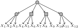
In this section, we applied the proposed algorithm to synthetic data to learn the latent hierarchical causal graph. Specifically, we considered different types of latent graphs and different sample sizes (with N = 2k, 5k, 10k), where structures are provided in Fig. 3 (Measurement Model and Latent Tree) and Fig. 1 (Hierarchical Model). The causal strength was generated uniformly from [-2.5, -0.5] ∪ [0.5, 2.5], and the noise term either follows a Gaussian distribution (represented by circular in the graph) or a uniform distribution U(-2, 2)
X1X2X3X4X5X6X7X8X9 X1X2X3X4X5X6X7X8 X9 X10X11 X12
| RCC | F1 ↑ | ||||||
|---|---|---|---|---|---|---|---|
| Algorithm | Ours | LNG | LHD | Ours | LNG | LHD | |
| 2k | 1.0 | 0.76 | 1.0 | 0.87 | 0.66 | 0.44 | |
| MM 5k | 1.0 | 0.86 | 1.0 | 1.0 | 0.86 | 0.51 | |
| 10k | 1.0 | 0.93 | 1.0 | 1.0 | 0.9 | 0.51 | |
| 2k | 0.98 | 0.36 | 0.96 | 0.87 | 0.21 | 0.63 | |
| LT 5k | 1.0 | 0.51 | 1.0 | 0.97 | 0.46 | 0.66 | |
| 10k | 1.0 | 0.6 | 1.0 | 1.0 | 0.55 | 0.66 | |
| 2k | 0.87 | 0.5 | 0.625 | 0.8 | 0.47 | 0.27 | |
| HM 5k | 0.91 | 0.56 | 0.68 | 0.86 | 0.52 | 0.38 | |
| 10k | 0.96 | 0.66 | 0.75 | 0.93 | 0.58 | 0.47 | |
(represented by the triangle in the graph). Each experiment was repeated ten times with randomly generated data.
We compare our method with the hierarchical-model-based method, Latent Hierarchical Causal Structure Discovery (LHD) [Huang et al., 2022] and Linear Non-Gaussian Latent Hierarchical Model (LNG) [Xie et al., 2022]. Furthermore, we used the percentage of correctly identified causal clusters (RCC) [Huang et al., 2022] and the F1 score over the latent structure to evaluate the performance.
The experimental results were reported in Table 1. Our method gives the best results on all types of graphs, indicating that it can handle not only the tree-based and measurementbased structures but also the latent hierarchical structure. The LHD method has a poor F1 score because it can not identify the causal direction between latent variables, while LNG has poor performance in two metrics because there is not enough non-Gaussianity to ensure the correctness of learned clusters.
6 Conclusion
We proposed new sufficient identifiability conditions of linear latent hierarchical causal structure. Theoretically, we show that under the mild restriction of the graph structure, i.e., the irreducible condition, and partial distribution condition, the linear latent hierarchical structure is identifiable. Our theoretical results relax the application scope of the linear latent hierarchical model and contribute to the general latent structure research. Future research directions include extending the one-factor model assumption to an n-factor model setting and allowing non-linear relations, existing techniques, e.g., [Kummerfeld et al., 2014; Zhang and Hyv¨arinen, 2009; Squires et al., 2022], may help to mitigate this issue.
Contribution Statement
Authors Zhengming Chen and Feng Xie contributed equally to this work.
Acknowledgements
This research was supported in part by National Key R&D Program of China (2021ZD0111501), National Science Fund for Excellent Young Scholars (62122022), Natural Science Foundation of China (61876043, 61976052), the major key project of PCL (PCL2021A12). FX acknowledges the support by National Natural Science Foundation of China (NSFC 62006051). We appreciate the comments from anonymous reviewers, which greatly helped to improve the paper.
@inproceedings{ijcai2023p397,
  title     = {Some General Identification Results for Linear Latent Hierarchical Causal Structure},
  author    = {Chen, Zhengming and Xie, Feng and Qiao, Jie and Hao, Zhifeng and Cai, Ruichu},
  booktitle = {Proceedings of the Thirty-Second International Joint Conference on
               Artificial Intelligence, {IJCAI-23}},
  publisher = {International Joint Conferences on Artificial Intelligence Organization},
  editor    = {Edith Elkind},
  pages     = {3568--3576},
  year      = {2023},
  month     = {8},
  note      = {Main Track},
  doi       = {10.24963/ijcai.2023/397},
  url       = {https://doi.org/10.24963/ijcai.2023/397},
}
TY - CPAPER TI - Some General Identification Results for Linear Latent Hierarchical Causal Structure AU - Chen, Zhengming AU - Xie, Feng AU - Qiao, Jie AU - Hao, Zhifeng AU - Cai, Ruichu T2 - Proceedings of the Thirty-Second International Joint Conference on Artificial Intelligence, IJCAI-23 PB - International Joint Conferences on Artificial Intelligence Organization PY - 2023 SP - 3568 EP - 3576 DO - 10.24963/ijcai.2023/397 UR - https://doi.org/10.24963/ijcai.2023/397 ER -Copied
Machine-readable versions of this paper, for tools and AI agents:





