
Unbiased Risk Estimator to Multi-Labeled Complementary Label Learning
Proceedings of the Thirty-Second International Joint Conference on Artificial Intelligence. Main Track. Pages 3732-3740.
https://doi.org/10.24963/ijcai.2023/415
Keywords
- Machine Learning: ML: Weakly supervised learning
- Machine Learning: ML: Classification
- Machine Learning: ML: Multi-label
Abstract
Multi-label learning (MLL) usually requires assigning multiple relevant labels to each instance. While a fully supervised MLL dataset needs a large amount of labeling effort, using complementary labels can help alleviate this burden. However, current approaches to learning from complementary labels are mainly designed for multi-class learning and assume that each instance has a single relevant label. This means that these approaches cannot be easily applied to MLL when only complementary labels are provided, where the number of relevant labels is unknown and can vary across instances. In this paper, we first propose the unbiased risk estimator for the multi-labeled complementary label learning (MLCLL) problem. We also provide an estimation error bound to ensure the convergence of the empirical risk estimator. In some cases, the unbiased estimator may give unbounded gradients for certain loss functions and result in overfitting. To mitigate this problem, we improve the risk estimator by minimizing a proper loss function, which has been shown to improve gradient updates. Our experimental results demonstrate the effectiveness of the proposed approach on various datasets.
- [Bartlett and Mendelson, 2002] Peter L. Bartlett and Sha- har Mendelson. Rademacher and gaussian complexities: Risk bounds and structural results. J. Mach. Learn. Res., 2111:224-240, 2002.
- [Boutell et al., 2004] Matthew R. Boutell, Jie-Bo Luo, Xi- Peng Shen, and Christopher M. Brown. Learning multi- label scene classification. Pattern Recognit., 37(9):1757- 1771, 2004.
- [Chou et al., 2020] Yu-Ting Chou, Gang Niu, Hsuan-Tien Lin, and Masashi Sugiyama. Unbiased risk estimators can mislead: A case study of learning with complementary la- bels. In Proceedings of the 37th International Conference on Machine Learning, pages 1929-1938, Virtual Event, 2020.
- [Elisseeff and Weston, 2001] André Elisseeff and Jason We- ston. A kernel method for multi-labelled classification. In Advances in Neural Information Processing Systems 14, pages 681-687, Vancouver, Canada, 2001.
- [Feng et al., 2020] Lei Feng, Takuo Kaneko, Bo Han, Gang Niu, Bo An, and Masashi Sugiyama. Learning with mul- tiple complementary labels. In Proceedings of the 37th International Conference on Machine Learning, pages 3072-3081, Virtual Event, 2020.
- [Fürnkranz et al., 2008] Johannes Fürnkranz, Eyke Hüllermeier, Eneldo Loza Mencía, and Klaus Brinker. Multilabel classification via calibrated label ranking. Machine learning, 73(2):133-153, 2008.
- [Gao and Zhang, 2021] Yi Gao and Min-Ling Zhang. Dis- criminative complementary-label learning with weighted loss. In Proceedings of the 38th International Conference on Machine Learning, pages 3587-3597, Virtual Event, 2021.
- [Gerych et al., 2021] Walter Gerych, Thomas Hartvigsen, Luke Buquicchio, Emmanuel Agu, and Elke A. Runden- steiner. Recurrent bayesian classifier chains for exact multi-label classification. In Advances in Neural Informa- tion Processing Systems 34, pages 15981-15992, Virtual Event, 2021.
- [Ghosh et al., 2017] Aritra Ghosh, Himanshu Kumar, and P. S. Sastry. Robust loss functions under label noise for deep neural networks. In Proceedings of the 31st AAAI Conference on Artificial Intelligence, pages 1919-1925, San Francisco, CA, 2017.
- [Ishida et al., 2017] Takashi Ishida, Gang Niu, Wei-Hua Hu, and Masashi Sugiyama. Learning from complementary la- bels. In Advances in Neural Information Processing Sys- tems 30, pages 5639-5649, Long Beach, CA, 2017.
- [Ishida et al., 2019] Takashi Ishida, Gang Niu, Aditya Kr- ishna Menon, and Masashi Sugiyama. Complementary- label learning for arbitrary losses and models. In Pro- ceedings of the 36th International Conference on Machine Learning, Proceedings of Machine Learning Research, pages 2971-2980, Long Beach, CA, 2019.
- [Li et al., 2017] Yun-Cheng Li, Yale Song, and Jie-Bo Luo. Improving pairwise ranking for multi-label image classifi- cation. In Proceedings of 2017 IEEE conference on com- puter vision and pattern recognition, pages 3617-3625, Honolulu, HI, 2017.
- [Ma et al., 2022] Ze-Yu Ma, Xiao Luo, Ying-Jie Chen, Mi- Xiao Hou, Jin-Xing Li, Ming-Hua Deng, and Guang- Ming Lu. Improved deep unsupervised hashing with fine- grained semantic similarity mining for multi-label image retrieval. In Proceedings of the 31st International Joint Conference on Artificial Intelligence, pages 1254-1260, Vienna, Austria, 2022.
- [Maltoudoglou et al., 2022] Lysimachos Maltoudoglou, An- dreas Paisios, Ladislav Lenc, Jirí Martínek, Pavel Král, and Harris Papadopoulos. Well-calibrated confidence measures for multi-label text classification with a large number of labels. Pattern Recognit., 122:108271, 2022.
- [Paszke et al., 2019] Adam Paszke, Sam Gross, Francisco Massa, Adam Lerer, James Bradbury, Gregory Chanan, Trevor Killeen, Ze-Ming Lin, Natalia Gimelshein, Luca Antiga, Alban Desmaison, Andreas Köpf, Edward Yang, Zachary DeVito, Martin Raison, Alykhan Tejani, Sasank Chilamkurthy, Benoit Steiner, Lu Fang, Jun-Jie Bai, and Soumith Chintala. Pytorch: An imperative style, high- performance deep learning library. In Advances in Neu- ral Information Processing Systems 32, pages 8024-8035, Vancouver, Canada, 2019.
- [Read et al., 2011] Jesse Read, Bernhard Pfahringer, Geoff Holmes, and Eibe Frank. Classifier chains for multi-label classification. Mach. Learn., 85(3):333-359, 2011.
- [Sun et al., 2019] Li-Juan Sun, Song-He Feng, Tao Wang, Cong-Yan Lang, and Yi Jin. Partial multi-label learning by low-rank and sparse decomposition. In Proceedings of the 33rd AAAI Conference on Artificial Intelligence, pages 5016-5023, Honolulu, HI, 2019.
- [Sun et al., 2022] Li-Juan Sun, Song-He Feng, Jun Liu, Geng-Yu Lyu, and Cong-Yan Lang. Global-local label correlation for partial multi-label learning. IEEE Trans. Multim., 24:581-593, 2022.
- [Tsoumakas et al., 2011] Grigorios Tsoumakas, Ioannis Katakis, and Ioannis P. Vlahavas. Random k-labelsets for multilabel classification. IEEE Trans. Knowl. Data Eng., 23(7):1079-1089, 2011.
- [Vapnik, 1991] Vladimir Vapnik. Principles of risk mini- mization for learning theory. In Proceedings of Advances in Neural Information Processing Systems (NIPS), pages 831-838, 1991.
- [Wu et al., 2018] Zhi-Rong Wu, Yuan-Jun Xiong, Stella X. Yu, and Da-Hua Lin. Unsupervised feature learning via non-parametric instance discrimination. In Proceedings of 2018 IEEE Conference on Computer Vision and Pattern Recognition, Salt Lake City, UT, 2018.
- [Xie and Huang, 2018] Ming-Kun Xie and Sheng-Jun Huang. Partial multi-label learning. In Proceedings of the 32nd AAAI Conference on Artificial Intelligence, pages 4302-4309, New Orleans, LA, 2018.
- [Xie and Huang, 2020] Ming-Kun Xie and Sheng-Jun Huang. Partial multi-label learning with noisy label identification. In Proceedings of 34th AAAI Conference on Artificial Intelligence, pages 6454-6461, New York, NY, 2020.
- [Xu et al., 2020] Yan-Wu Xu, Ming-Ming Gong, Jun-Xiang Chen, Tong-Liang Liu, Kun Zhang, and Kayhan Bat- manghelich. Generative-discriminative complementary learning. In Proceedings of the 34th AAAI Conference on Artificial Intelligence, pages 6526-6533, New York, NY, 2020.
- [Xu et al., 2022a] Cheng-Yin Xu, Zeng-Hao Chai, Zheng- Zhuo Xu, Chun Yuan, Yan-Bo Fan, and Jue Wang. Hyp 2 loss: Beyond hypersphere metric space for multi-label im- age retrieval. In Proceedings of the 30th ACM Interna- tional Conference on Multimedia, pages 3173-3184, Lis- boa, Portugal, 2022.
- [Xu et al., 2022b] Ning Xu, Cong-Yu Qiao, Jia-Qi Lv, Xin Geng, and Min-Ling Zhang. One positive label is suffi- cient: Single-positive multi-label learning with label en- hancement. In Advances in Neural Information Processing Systems 35, in press, 2022.
- [Yu et al., 2018a] Guo-Xian Yu, Xia Chen, Carlotta Domeni- coni, Jun Wang, Zhao Li, Zi-Li Zhang, and Xin-Dong Wu. Feature-induced partial multi-label learning. In Proceed- ings of 2018 IEEE International Conference on Data Min- ing, pages 1398-1403, Singapore, 2018.
- [Yu et al., 2018b] Xi-Yu Yu, Tong-Liang Liu, Ming-Ming Gong, and Da-Cheng Tao. Learning with biased comple- mentary labels. In Proceedings of the 15th European Con- ference on Computer Vision, pages 69-85, Munich, Ger- many, 2018.
- [Zhang and Wu, 2015] Min-Ling Zhang and Lei Wu. Lift: Multi-label learning with label-specific features. IEEE Trans. Pattern Anal. Mach. Intell., 37(1):107-120, 2015.
- [Zhang and Zhou, 2006] Min-Ling Zhang and Zhi-Hua Zhou. Multilabel neural networks with applications to functional genomics and text categorization. IEEE transactions on Knowledge and Data Engineering, 18(10):1338-1351, 2006.
- [Zhang and Zhou, 2007] Min-Ling Zhang and Zhi-Hua Zhou. ML-KNN: A lazy learning approach to multi-label learning. Pattern Recognit., 40(7):2038-2048, 2007.
- [Zhang and Zhou, 2014a] Min-Ling Zhang and Zhi-Hua Zhou. A review on multi-label learning algorithms. IEEE Trans. Knowl. Data Eng., 26(8):1819-1837, 2014.
- [Zhang and Zhou, 2014b] Min-Ling Zhang and Zhi-Hua Zhou. A review on multi-label learning algorithms. IEEE Trans. Knowl. Data Eng., 26(8):1819-1837, 2014.
- [Zhang et al., 2018] Min-Ling Zhang, Yu-Kun Li, Xu-Ying Liu, and Xin Geng. Binary relevance for multi-label learn- ing: an overview. Frontiers Comput. Sci., 12(2):191-202, 2018.
- [Zhang et al., 2022] Yu Zhang, Zhi-Hong Shen, Chieh-Han Wu, Bo-Ya Xie, Jun-Heng Hao, Ye-Yi Wang, Kuan-San Wang, and Jia-Wei Han. Metadata-induced contrastive learning for zero-shot multi-label text classification. In Proceedings of the ACM Web Conference 2022, pages 3162-3173, Virtual Event, 2022.
- [Zhao et al., 2021] Wen-Ting Zhao, Shu-Feng Kong, Jun- Wen Bai, Daniel Fink, and Carla P. Gomes. HOT-VAE: learning high-order label correlation for multi-label clas- sification via attention-based variational autoencoders. In Proceedings of 35th AAAI Conference on Artificial Intelli- gence, pages 15016-15024, Virtual Event, 2021.
- [Zhou, 2018] Zhi-Hua Zhou. A brief introduction to weakly supervised learning. National Science Review, 5(1):44-53, 2018.
- [Zhou, 2022] Zhi-Hua Zhou. Open-environment machine learning. National Science Review, 9(8):nwac123, 2022.
References were extracted automatically from the PDF and may contain errors.
Full text extracted automatically from the PDF; figures, tables and equations may differ. The PDF is the version of record.
1 Introduction
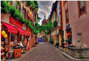
Multi-label learning (MLL) is a method of training a classifier that can predict multiple labels for an unseen instance simultaneously [Zhang and Zhou, 2014a]. It has been widely used in open-environment [Zhou, 2022] and various realworld applications such as text categorization [Maltoudoglou et al., 2022; Zhang et al., 2022] and image retrieval [Xu et al., 2022a; Ma et al., 2022]. However, collecting accurate multilabeled data can be challenging due to the difficulty of identifying small objects or complex semantic labels in complex images, as well as the unknown number of relevant labels. This requires a significant amount of labeling effort as annotators need to exercise caution and possess specialized knowledge. Precisely annotating images, such as the one shown in
∗Corresponding author
The relevant label
set
cloud plant house
balloon
people Europe
…
Complementary label Not "river"
Figure 1: An example. The image is labeled with a variety of relevant labels including "cloud", "plant", "house", "balloon", "people", "Europe", and others. The complementary label of this image is "river". Labeling the image with the label "Europe" requires specialized knowledge as it is a complex semantic label that is challenging to annotate. On the other hand, the label "people" refers to a small object that is difficult to spot, as it is highlighted by a blue box in the image.
Fig. 1, requires a high level of attention and expertise, particularly when it comes to identifying the easily overlooked label "people" or specific geographic location label "Europe". Additionally, accurate identification of other relevant labels involves a thorough examination of each label within the entire label space.
To release the laborious of collecting multi-labeled data, we study the setting of multi-labeled complementary label learning (MLCLL) that could significantly reduce labeling effort, whose goal is to learn a multi-labeled classifier that can assign relevant labels for unseen instances. In MLCLL, each instance is associated with a single complementary label that specifies an irrelevant label of the instance. Obviously, providing weakly supervised information - complementary labels - releases annotation costs since selecting a complementary label does not need one-by-one checking of the entire label space and prior knowledge. For example, selecting the label "river" as the complementary label for the image in Fig. 1 is much easier than selecting all relevant labels.
Complementary label learning (CLL) is a method previously proposed for multi-class scenarios by Ishida et al. [2017]. Ishida et al. [2019] proposed an unbiased risk estimator by deriving a transition matrix using the fact that the complementary label is uniformly sampled besides the only one relevant label, such that any loss function can be used. With such an unbiased risk estimator, the classification risk of fully-supervised learning can be evaluated on CLL training data, enabling empirical risk minimization [Vapnik, 1991]. CLL problems are further studied for biased complementary labels [Yu et al., 2018b], generative adversarial network [Xu et al., 2020], multiple complementary labels [Feng et al., 2020], improved gradient estimation [Chou et al., 2020], or easing the dependence on estimating the transition matrix [Gao and Zhang, 2021]. These existing works are based on the fact that only one relevant label exists for multi-class cases, and most solutions are strongly dependent on the known number of irrelevant labels. They cannot be used to solve the MLCLL problem, due to the unknown number of relevant labels in MLL given only a complementary label.
To address the MLCLL problem, we first propose an unbiased risk estimator that utilizes the distribution of complementary data to approximate the distribution of fullysupervised data under certain assumptions. We also establish an estimation error bound for this estimator, guaranteeing that the classifier learned from complementary labeled data will converge to the optimal one from fully-supervised MLL. Furthermore, we analyze the impact of cross-entropy loss on learning when a crucial assumption is not met and propose a gradient-friendly loss function to prevent overfitting. Our experimental results demonstrate the effectiveness of the proposed risk minimization methods.
Our contributions are summarized as follows:
- The proposal of an unbiased risk estimator for MLCLL and the derivation of an estimation error bound to ensure that the classifier learned from complementary labeled data is similar to the optimal one learned from fullysupervised MLL
- The improvement of the risk estimator by using a gradient-friendly loss function to prevent overfitting, which can occur when a crucial assumption does not hold.
The rest of this paper is organized as follows. Section 2 briefly reviews related work. We introduce our proposed approach and the gradient-friendly loss function Section 3 and 4 respectively. Section 5 describes experimental results, and Section 6 gives the conclusion.
2 RelatedWork
In MLL, the main challenge is that the number of the output space grows exponentially as the number of labels increases [Zhang and Zhou, 2014b]. There are three routes to cope with MLL problems: first-order approach [Zhang et al., 2018; Zhang and Zhou, 2007], second-order approach [Elisseeff and Weston, 2001; F¨urnkranz et al., 2008] and high-order approach [Read et al., 2011; Tsoumakas et al., 2011]. The firstorder approaches decompose MLL problems into a series of binary classification problems to solve [Zhang et al., 2018; Boutell et al., 2004]. Subsequently, Zhang et al. [Zhang and Zhou, 2014b; Zhang and Wu, 2015] revealed that label correlations exist in multi-labeled data, more and more studies consider label correlations to address MLL problems [Gerych et al., 2021; Li et al., 2017]. Among them, the secondorder approaches consider label correlations between label pairs [F¨urnkranz et al., 2008; Zhang and Zhou, 2006; Li et al., 2017]. Beyond the second-order relationship, the highorder approaches pay attention to exploring label correlations among label sets [Read et al., 2011; Gerych et al., 2021; Zhao et al., 2021].
In practice, collecting precisely multi-labeled data is difficult because labeling information is often incomplete [Xu et al., 2022b]. A weakly supervised framework - partial multilabel learning (PML) - is designed to alleviate the pain of collecting precisely labeled data [Zhou, 2018]. PML was firstly proposed by Xie and Huang [2018], where each instance is associated with a set of candidate labels that consists of relevant labels and irrelevant (noisy) labels. Existing PML approaches handle PML problems according to the assumption that noisy labels only compose a small portion of candidate labels [Sun et al., 2022; Xie and Huang, 2020; Sun et al., 2019; Yu et al., 2018a]. Then, these approaches use the matrix factorization technique to decompose the candidate label matrix into the low-rank multi-label matrix and the sparse noisy label matrix to solve PML problems.
CLL was first applied in multi-class learning [Ishida et al., 2017], whose emergence significantly reduces annotation costs in multi-class learning. CLL aims to recover relevant labels from complementary labels. Ishida et al. [2019] used uniformly sampled complementary labels to derive an unbiased risk estimator that is available for arbitrary loss functions to solve the CLL problem. In addition, studies of CLL problems further involve biased complementary labels, whose implementation depends on estimating a transition matrix [Yu et al., 2018b]. To ease the dependence on estimating transition matrix, Gao and Zhang [2021] designed a discriminative way to directly model the probabilities of complementary labels. Moreover, multiple complementary labels were proposed to make the learning process have more labeling information compared with one complementary label [Feng et al., 2020].
Compared with PML, MLCLL considers the hardest version of this problem - a high-noise PML problem, where the candidate label set of an instance is all labels other than its complementary label. In this case, existing PML approaches may be inapplicable for MLCLL since their implementations are based on the assumption of few noisy included in candidate labels. For CLL, existing approaches are accomplished by the fact that each instance has one relevant label in multiclass learning and irrelevant labels are known. However, the number of relevant labels is unknown and can vary across instances in MLL, which leads to CLL approaches that could not handle MLCLL problems.
3 The Proposed Approach
In this section, we first introduce notations and problem setting (Sec. 3.1) and the recovery of data distribution given complementary labels (Sec. 3.2). Then, we propose an unbiased risk estimator with its estimation error bound (Sec. 3.3).
3.1 Preliminaries
Let X ⊂ Rd be the feature space with d dimensions and Y = {1, 2, 3, . . . ,K} be the label space with K (K > 2)
possible labels. In MLL, an instance x ∈ X with its relevant label set Y ⊆ Y is drawn from the unknown joint probability distribution p(x, Y ). Given fully supervised data, MLL aims to learn a classifier f : X ↦→ [0, 1]K by minimizing the following classification risk:
where
Denoting the j-th prediction of f as fj which estimates p(j = 1|x), ℓj(x) and ¯ ℓj(x) calculate the loss of fj(x) respectively on relevant and irrelevant labels. Specially, when ℓj(x) = -log(fj(x)) and ¯ ℓj (x) = - log(1 - fj (x)), L(f (x), Y ) is the popular BCE loss. L(f(x), Y ) is not limited to BCE loss only. The mean absolute error (MAE) loss can also be used, resulting in ℓj(x) = 1 - fj(x) and ¯ ℓj (x) = fj (x).
For the MLCLL problem studied in this paper, fully supervised data is unavailable. Instead, ¯D = {(xi, ¯ yi)}ni=1 containing n training instances is given, where ¯ yi ∈ {Y - Yi} is the complementary label of xi ∈ X. Even given the complementary training set, the goal of MLCLL is still to learn a multi-labeled classifier f : X ↦→ [0, 1]K , i.e., the same goal as fully supervised MLL. As (x, Y ) follows a distribution p(x, Y ), (x, ¯ y) also follows a distribution, which is denoted as ¯ p(x, ¯ y) on which ¯D is drawn. In the next subsection, we will construct the relationship between p(x, Y ) and ¯ p(x, ¯ y) under some assumptions, and propose one scenario which guarantees assumptions to hold.
3.2 Recovering the Distribution
Without any additional knowledge, it is naturally difficult to construct the relationship between p(x, Y ) and ¯ p(x, ¯ y), especially when the number of unlabeled data is unknown. To enable the construction, below we provide some assumptions.
Assumption 1. Instance-Independent Assumption: Given the complementary label ¯ y, the relevant label set Y is independent of x, i.e. p(Y |¯ y) = p(Y |x, ¯ y).
Assumption 1 is motivated by existing works on complementary labels [Yu et al., 2018b; Feng et al., 2020; Ishida et al., 2019], which assumes that the complementary label is conditionally independent of x given relevant labels. This assumption does not necessarily lead to the prediction of p(Y |x), because the information on complementary labels in MLL is not complete with only one complementary label provided. Information on other complementary labels and learning on x are still essential. The following result provided a conclusion based on Assumption 1.
Lemma 1. Under Assumption 1, ∑K¯ y=1, ¯ y /∈Y ¯ p(x, ¯ y) 2K-1-1 is a valid probability mass function with respect to x and Y , i.e., it is non-negative and
The proof is stated in Appendix A. We then give another assumption, which describes the relationship between Y and ¯ y.
Assumption 2. UniformGeneration Assumption:
Assumption 2 provides the information on how complementary labels can contribute to the prediction of Y , i.e., Y can be any subset of Y - ¯ y -∅ with uniform probability. This is a strong assumption for the difficult MLCLL problem, which implies that the complementary label ¯ y will contribute to learning no more than an irrelevant label. Such an assumption will be a necessary ground to give the unbiased risk estimation for MLCLL in Section 3.3, and will discuss an alternative solution in Section 4 if such an assumption does not hold.
With these assumptions, the following result gives the relationship between p(x, Y ) and ¯ p(x, ¯ y).
Theorem 1. Under Assumption 1 and Assumption 2,
It has been verified in Lemma 1 that the right side of Eq. (5) forms a valid probability mass function under Assumption 1.
3.3 Unbiased Risk Estimator
An unbiased risk estimator enables the classification risk of fully-supervised MLL to be evaluated on the given MLCLL training data. The following result shows an unbiased risk estimator of the fully supervised MLL classification risk R(f) defined in Eq. (1).
Theorem 2. With p(x, Y ) defined in Eq. (5) and R(f) defined in Eq. (1), R(f) = ¯R(f), where ¯R(f) = E¯ p(x, ¯ y)[ ¯ L(f(x), ¯ y)] is the expected risk on complementary data, and
The proof is proved in Appendix B. Theorem 2 shows that the fully-supervised classification risk can be estimated using the complementary labels by the unbiased estimator ¯R(f), with the corresponding complementary loss function defined in Eq. (6). Eq. (6) shows that the complementary loss gives low confidence in treating other labels as either relevant or irrelevant with smaller-than-one weights for them.
Estimation Error Bound. With Theorem 2, the expected risk ¯R(f) can be approximated by its empirical estimation ¯Rn(f), which is¯Rn(f) = 1n n∑ i=1 ¯ L(f(xi), ¯ yi). (7)
Denote F as the hypothesis class and Gj = {g : x ↦→ fj(x)|f ∈ F} as the functional space for the label j ∈
Algorithm 1 MLCLL with the GDF loss
Input:
¯D = {(xi, ¯ yi)}ni=1 : the training data;
E : the number of epochs;
A : an external stochastic optimization algorithm
Output:
θ : model parameter for f(x; θ)
- 1: for t = 1 to E do
- 2: Let L be the risk, L = 1n ∑ni=1 ¯ LGDF(f(xi), ¯ yi);
- 3: Set gradient -▽θ L;
- 4: Update θ by A;
- 5: end for
Y. Rn(Gj) gives the Rademacher Complexity [Bartlett and Mendelson, 2002] of Gj, defined as Rn(Gj) = Ex,σ [supg∈Gj 1n ∑ni=1 g(xi)]. We further denote fn ∈ F and f ∗ ∈ F as the minimizers of ¯Rn(f) and R(f) respectively. Based on these notations, we give the estimation error bound.
Theorem 3. Suppose M = supx∈X,f∈F ¯ L(f(x), ¯ y). For any j ∈ Y, assuming ℓj(x) and ¯ ℓj(x) are β+-Lipschitz and β--Lipschitz with respect to f(x) respectively. For any δ, with the probability at least 1 - δ,
The proof is shown in Appendix C. Theorem 3 demonstrates that the empirical risk minimizer converges to the true risk minimizer as n →∞. It also demonstrates the impact of K on learning complementary labeled problems.
4 Gradient Descent Friendly Loss
In the above section, necessary assumptions are made for giving an unbiased risk estimator for the MLCLL problem, especially Assumption 2, which assumes that there exists no additional bias in learning besides that ¯ y is an irrelevant label. In this section, we will investigate the situation that Assumption 2 does not hold from the perspective of the loss function and give a moderated solution.
Our proposed complementary loss function Eq. (6) is eligible to accommodate any loss functions. If we use the popular BCE loss, we have
Motivated by [Chou et al., 2020] which concluded that gradient estimation is important for weakly supervised learning, we further give the gradient of ¯ LBCE with respect to θ, which is learnable parameters for fj(x):
The calculation in Eq. (10) is divided into two parts: on the complementary label ¯ y and non-complementary labels Y - ¯ y. On the complementary label, the gradient descent favors a prediction of zero for f¯ y(x; θ). However, serious overfitting can happen regarding the punishment on non-complementary labels Y - ¯ y if Assumption 2 does not hold, i.e., ¯ y provides some bias in learning other labels.
To give a simple example, imagine there is another label ys which is similar to ¯ y, such that its prediction fys (x; θ) will be close to the prediction on f¯ y(x; θ), i.e., zero. When fys (x; θ) = 0 or close to zero, w+ in Eq. (10) will become ∞, resulting in ∞ gradient although the prediction fys is already close to the groundtruth. In another example, when a label yd is absolutely exclusive of ¯ y, its close-to-groundtruth prediction should be close to one, resulting in an infinity w-, still an ∞ gradient despite that the prediction is close to groundtruth. These two naive examples could demonstrate that if Assumption 2 is violated, serious overfitting could happen when using the proposed unbiased risk estimator.
To mitigate the overfitting caused due to violating Assumption 2, we design a new gradient by using the ¯ y part in Eq. (10), but a modification on the gradient of the Y - ¯ y part. Such a gradient is potentially calculated from a GradientDescent-Friendly (GDF) loss function and shown as
Eq. (11) achieves a kind of gradient that will enable any label belonging to Y - ¯ y to have a prediction higher than the prediction on the complementary label, i.e., achieving a good ranking effect. When the label absolutely exclusive from ¯ y exists, such a gradient will favor the prediction to be close to one. It seems that the problem still remains if there is any label similar to ¯ y exists, however, the learning on ¯ y will provide a way of balancing the learning of these two labels, and a good ranking performance can still be achieved in MLL metrics such as ranking loss or average precision. In Eq. (11), we remove all weights related to K to make the gradients caused by individual labels have uniform weights in case one label dominates the learning.
The corresponding loss function of Eq. (11) is
The procedure for optimizing the GDF loss is shown in Algorithm 1. We will show in the next section how optimizing Eq. (12) can mitigate overfitting and improve performance.
| Methods | MLL | PML | CLL | Unbounded | Bounded | |||
|---|---|---|---|---|---|---|---|---|
| ML-KNN | LIFT | fpml | PML-LRS | L-UW | BCE | MAE | GDF | |
| One Error↓ | ||||||||
| bookmark Corel16k delicious mediamill eurlex dc eurlex sm scene yeast | .801±.006• .736±.054• .592±.017• .198±.020• .790±.033• .667±.017• .692±.029• .297±.028• | .649±.015• .789±.044• .533±.014• .187±.019 .759±.024• .674±.013• .605±.022• .284±.027• | .885±.019• .816±.023• .617±.017• .188±.019 .920±.024• .868±.032• .815±.026• .251±.023 | .584±.004• .730±.000• .452±.007• .200±.002• .517±.013• .457±.005• .540±.022• .738±.097• Ranking Loss↓ | .504±.008• .703±.058 .482±.018• .188±.019 .609±.024• .552±.011• .764±.023• .253±.022 | .568±.006• .798±.019• .490±.011• .190±.014• .575±.019• .534±.012• .449±.031• .277±.016• | .613±.011• .702±.053 .467±.019• .188±.019 .906±.010• .834±.008• .805±.021• .251±.023 | .483±.007 .706±.053 .426±.012 .184±.018 .459±.015 .400±.010 .383±.020 .249±.024 |
| mediamill eurlex dc eurlex sm scene yeast bookmark Corel16k eurlex sm | .405±.047 .711±.010• .426±.009• | .480±.010• .350±.033• .511±.004• .710±.009• .429±.016• .425±.012• | .457±.006• .709±.012• .285±.026• | .464±.018• .423±.006 .584±.004• | .604±.005• .434±.047 .554±.006• .717±.012• .475±.008• | .544±.005• .343±.017• .544±.005• .765±.005◦ .524±.012• | .494±.008• .426±.040 .567±.006• .715±.012• .267±.009• .288±.003• | .619±.006 .429±.044 .586±.004 .732±.007 .623±.009 |
| bookmark Corel16k delicious | .348±.006• .328±.045• .398±.004• .200±.014• .283±.008• .322±.007• .340±.030• .247±.011• .383±.006• | .310±.007• .392±.026• .298±.012• | .420±.031• .438±.008• .206±.019• .470±.037• .472±.034• .504±.024• | .303±.005 .305±.002• .160±.001◦ .179±.006• .238±.004• | .196±.007 .301±.039 .319±.005• .193±.020• .267±.015• .329±.005• | .260±.005• .400±.016• .336±.003• .157±.009◦ .216±.017• | .316±.032 .305±.004• .192±.019• .437±.008• .461±.006• | .307±.040 .292±.005 .174±.013 .161±.005 .209±.006 .153±.009 .219±.013 |
| Precision↑ | ||||||||
| delicious | .383±.003• .202±.015• .294±.012• .333±.013• .289±.019• | .468±.019• | .260±.004• | .301±.008• | .196±.005 | |||
| mediamill eurlex dc | .417±.018• | .233±.012• .267±.018• .325±.021• .240±.028• | .258±.006• .616±.009• | .457±.018• .252±.012• .525±.017• | .273±.014• .184±.019• .563±.014• | .492±.023• | .658±.010 | |
| Average | ||||||||
| .250±.015• | .238±.014• | |||||||
| .534±.004• | ||||||||
| scene yeast | .487±.006• .543±.023• .677±.018• | .600±.016• .636±.016• | .417±.020• .688±.016• | .580±.002• .748±.001◦ .637±.010• .459±.031• | .463±.018• .679±.016• | .717±.022• .679±.015• | .429±.018• .693±.017• | .759±.012 .712±.018 |
MAE loss is another widely used loss function, which is shown to be less likely to overfit but slower at convergence [Ghosh et al., 2017]. Formally, the MLCLL corresponding MAE loss and its gradients are
and
Eq. (14) shows the reason why the ¯ LMAE is less likely to overfit but slower in convergence compared to the ¯ LBCE. By comparing Eqs. (10), (14) and (11), we can see that the GDF loss is a trade-off between the MAE one and the BCE one from the perspective of the gradient. The relationship between ¯ LGDF and ¯ LMAE can be further shown by the fact that ¯ LMAE ≤ ¯ LGDF. The empirical comparison of optimizing these three loss functions is shown in Section 5.
5 Experiments
In this section, we conduct experiments to evaluate the performance of the unbiased risk estimator with various loss functions and our proposed GDF loss. Here, we adopt five MLL criteria, including ranking loss, hamming loss, one error, coverage and average precision, to measure the performance of approaches. For average precision, the greater the value, the better the performance, while for the remaining four criteria, the smaller the values the better the performance. We use PyTorch [Paszke et al., 2019] and NVIDIA TITAN RTX to implement our experiments, where the code is available at https://github.com/GaoYi439/GDF.
5.1 Experimental Settings
Datasets & pre-processing. We use eight widely-used MLL datasets to experiments 1 , where we adopt two preprocessing ways to process datasets to verify the performance of the proposed approach. The first way follows Xie et al. [2018; 2020], rare labels and instances being relevant to these rare labels are removed for datasets with more than 15 labels, whose labels are kept under 15. Datasets use the first way to process, where each instance is associated with one complementary label. The second way keeps the original number of labels for datasets, while the number of complementary labels per instance is half the original number of labels in datasets. The descriptions of these datasets are shown in Appendix D.
1 Publicly available at https://mulan.sourceforge.net/datasetsmlc.html.
Baselines. We adopt two PML approaches (fpml [Yu et al., 2018a] and PML-LRS [Sun et al., 2019]) as baselines, which use candidate labels (Y \ ¯ y) to learn. Similarly, a CLL approach, L-UW [Gao and Zhang, 2021], is used in our experiments. Due to that L-UW is applied in multi-class learning, we use the Sigmoid layer and BCE loss to replace the Softmax layer and cross-entropy loss respectively, and help it suit the MLCLL problem. In addition, ML-KNN [Zhang and Zhou, 2007] and LIFT [Zhang and Wu, 2015] are two MLL approaches, which are absorbed to compare with our approach. They deal with MLCLL by taking all candidate labels (Y \ ¯ y) of instances as possible labels. To verify the feasibility of theoretical analysis in Section 4, we use the BCE loss ¯ LBCE andMAE loss ¯ LMAE to our empirical risk estimator Eq. (7) as baselines. The proposed GDF loss is inserted into Eq. (7).
Setup. We adopt the linear model as the predictive model for fair comparisons and apply SGD with momentum 0.9 for optimization. We set batch-size and training epoch as 256 and 200 respectively. Weight decay is set as 10-3 and learning rate is selected from {10-1 , 10-2 , 10-3 }, where the learning rate is multiplied by 0.1 at 100 and 150 epochs [Wu et al., 2018]. We apply the same model and hyper-parameters of ours for L-UW, ¯ LBCE and ¯ LMAE. Ten-fold cross-validation is used to evaluate the performance of all approaches. Here, training data is only equipped with complementary labels and test data associated with the sets of relevant labels is used to verify the performance of approaches. We adopt the mean and standard deviation (std) of five criteria. ↓ / ↑ indicates that criteria are smaller/larger, the performance is better.
5.2 Main Empirical Results
Results. Table 1 reports one error, ranking loss, and average precision of various approaches over eight datasets (the results of hamming loss and coverage are shown in Appendix D). Here, all datasets are processed by the first pre-processing way, where each instance is associated with one complementary label. As shown in Table 1, GDF outperforms the most approaches on eight datasets. Specifically, we improve upon the best baseline on one error, ranking loss, and average precision by 0.066, 0.031, and 0.099 respectively on scene and eurlex sm datasets. This indicates the effectiveness of our proposed approach GDF to solve the MLCLL problem.
Moreover, GDF achieves comparable results on three criteria against two MLL approaches over all datasets. For example, GDF on average precision are significantly superior to ML-KNN and LIFT by 0.241 and 0.229 respectively on eurlex dc dataset. This is because our approach is more suitable for dealing with complementary labeled data than MLL
| Methods | MLL | PML | CLL | Bounded | GDF | |
|---|---|---|---|---|---|---|
| ML-KNN | fpml | PML-LRS | L-UW | MAE | ||
| Ranking Loss↓ | ||||||
| Corel16k delicious eurlex dc eurlex sm | .276±.043 .235±.002• .267±.004• .173±.004• | .286±.054 .204±.002• .263±.005• .208±.007• | .281±.013 .261±.009• .243±.003• .170±.002• | .293±.052• .195±.002• .252±.006• .167±.004• | .307±.051• .201±.002• .248±.008• .167±.003• | .286±.036 .186±.002 .239±.005 .159±.004 |
| Average Precision↑ | ||||||
| Corel16k delicious eurlex dc eurlex sm | .224±.042• .205±.003• .300±.011 .407±.009• | .238±.045 .201±.002• .179±.007• .204±.004• | .223±.009• .232±.001• .299±.003• .413±.002 | .244±.046 .235±.003• .278±.006• .370±.006• | .245±.046 .234±.003• .233±.008• .321±.009• | .240±.042 .299±.004 .300±.008 .413±.008 |
approaches. GDF achieves similar or better performance to PML approaches. Especially, the average precision of GDF is 0.418 higher than fpml on eurlex dc dataset, which shows that our approach can work well on MLCLL with the highnoisy problem compared with PML approaches.
Results of GDF shown in Table 1 outperform L-UW on all datasets, which indicates that the CLL approach can not enough handle the MLCLL problem. This is because their implementations depend on the assumption of one relevant label per instance, while the number of relevant labels for each instance is unknown in MLL. That leads to CLL approaches could not hold the relationship of multiple relevant labels and complementary labels in MLCLL. In addition, we observe that the unbounded loss BCE used to the empirical risk estimator Eq. (7) is inferior to our proposed GDF loss in most cases, which proves that GDF is indeed better than the unbounded one in MLCLL. Accordingly, experimental results of the empirical risk estimator Eq. (7) with MAE loss on three criteria are lower than ours in all datasets, which further proves the effectiveness of our proposed strategy - minimizing the empirical risk estimator by the GDF loss.
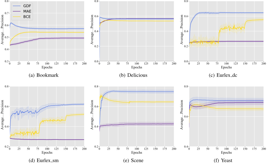
Effect of the gradient descent friendly loss GDF. Fig. 2 shows average precision of BCE loss, MAE loss and GDF loss on various datasets over 200 epochs, where six datasets both adopt the first pre-processing way to process and each instance is associated with one complementary label. As can be seen from Fig. 2, the curve of MAE loss is lower than that of BCE loss, but MAE loss is more stable than BCE loss in Fig. 2. It clearly illustrates the advantages and disadvantages of MAE loss: the bounded loss MAE is more robust for noisy data than unbounded loss BCE, while its convergence rate is inferior to the unbounded loss [Ghosh et al., 2017]. In addition, we observe that the curve of our proposed GDF loss is higher than these of the unbounded loss BCE and the bounded loss MAE, which demonstrates the effectiveness of our approach. Specifically, the curve of GDF loss shows that our approach has both the robustness of the bounded loss MAE and the superior convergence of the unbounded loss BCE. This demonstrates that removing the easily caused overfitting part of BCE loss to design GDF loss is a reasonable strategy in MLCLL to improve performance of our approach, which also confirms that GDF loss to optimize in MLCLL brings benefits to gradient update.
5.3 Additional Experiments
Table 2 shows ranking loss and average precision of different approaches on four datasets that are adopted the second preprocessing way to process, the remaining experimentations of three criteria are shown in Appendix D. Here, each dataset keeps the original number of labels and complementary labels given per instance is half of L(S) (the number of labels). In Table 2, the proposed approach achieves comparable performance to excellent baselines on four datasets, which indicates that GDF loss can also work on datasets with the original label space. Specifically, results of fpml and PML-LRS are inferior to GDF loss, which indicates that PML approaches depending on the assumption of sparse noisy labels can not deal with the high-noisy label problem of MLCLL. Table 2 illustrates that GDF loss outperforms L-UW, which proves that the proposal is better than the CLL approach in tackling the relationship between multiple relevant labels and complementary labels. GDF loss obtains better performance compared with MAE loss, which indicates that the proposed loss function designed by improving gradient updates can also deal with the multiple complementary-label problem.
6 Conclusion
In this paper, we study the setting of MLCLL, which aims to learn a multi-labeled classifier from complementary labeled data. To solve this problem, we propose an unbiased risk estimator with an estimation error bound, which supports that the learned risk minimizer from complementary labeled data converges to the optimal one of fully supervised MLL. Although our unbiased risk estimator has no restrictions on loss functions, it will produce unbounded gradients if certain unbounded loss functions are used and result in overfitting. To alleviate this issue, we design GDF loss to prevent the overfitting problem and find that it brings benefits to gradient updates. We verify the effectiveness of the proposed upper bound loss on various datasets.
Acknowledgments
The authors wish to thank the anonymous reviewers for their helpful comments and suggestions. This work was supported by the National Science Foundation of China (62225602) and the UQ Cyber Research Seed Funding (2021-R3). We thank the Big Data Center of Southeast University for providing the facility support on the numerical calculations in this paper.
@inproceedings{ijcai2023p415,
  title     = {Unbiased Risk Estimator to Multi-Labeled Complementary Label Learning},
  author    = {Gao, Yi and Xu, Miao and Zhang, Min-Ling},
  booktitle = {Proceedings of the Thirty-Second International Joint Conference on
               Artificial Intelligence, {IJCAI-23}},
  publisher = {International Joint Conferences on Artificial Intelligence Organization},
  editor    = {Edith Elkind},
  pages     = {3732--3740},
  year      = {2023},
  month     = {8},
  note      = {Main Track},
  doi       = {10.24963/ijcai.2023/415},
  url       = {https://doi.org/10.24963/ijcai.2023/415},
}
TY - CPAPER TI - Unbiased Risk Estimator to Multi-Labeled Complementary Label Learning AU - Gao, Yi AU - Xu, Miao AU - Zhang, Min-Ling T2 - Proceedings of the Thirty-Second International Joint Conference on Artificial Intelligence, IJCAI-23 PB - International Joint Conferences on Artificial Intelligence Organization PY - 2023 SP - 3732 EP - 3740 DO - 10.24963/ijcai.2023/415 UR - https://doi.org/10.24963/ijcai.2023/415 ER -Copied
Machine-readable versions of this paper, for tools and AI agents:





