
Contrastive Learning and Reward Smoothing for Deep Portfolio Management
Proceedings of the Thirty-Second International Joint Conference on Artificial Intelligence. Main Track. Pages 3966-3974.
https://doi.org/10.24963/ijcai.2023/441
Keywords
- Machine Learning: ML: Relational learning
- Machine Learning: ML: Representation learning
- Machine Learning: ML: Reinforcement learning
Abstract
In this study, we used reinforcement learning (RL) models to invest assets in order to earn returns. The models were trained to interact with a simulated environment based on historical market data and learn trading strategies. However, using deep neural networks based on the returns of each period can be challenging due to the unpredictability of financial markets. As a result, the policies learned from training data may not be effective when tested in real-world situations. To address this issue, we incorporated contrastive learning and reward smoothing into our training process. Contrastive learning allows the RL models to recognize patterns in asset states that may indicate future price movements. Reward smoothing, on the other hand, serves as a regularization technique to prevent the models from seeking immediate but uncertain profits. We tested our method against various traditional financial techniques and other deep RL methods, and found it to be effective in both the U.S. stock market and the cryptocurrency market. Our source code is available at https://github.com/sophialien/FinTech-DPM.
- [Almahdi and Yang, 2017] Saud Almahdi and Steve Y Yang. An adaptive portfolio trading system: A risk-return port- folio optimization using recurrent reinforcement learning with expected maximum drawdown. Expert Systems with Applications, 87:267-279, 2017.
- [Buehler et al., 2019] Hans Buehler, Lukas Gonon, Josef Te- ichmann, and Ben Wood. Deep hedging. Quantitative Fi- nance, 19(8):1271-1291, 2019.
- [Chen et al., 2020] Ting Chen, Simon Kornblith, Moham- mad Norouzi, and Geoffrey Hinton. A simple framework for contrastive learning of visual representations. In In- ternational conference on machine learning, pages 1597- 1607, 2020.
- Thomas M Cover. Universal portfolios. In The Kelly Capital Growth Investment Criterion: Theory and Practice, pages 181-209, 2011.
- [Crawshaw, 2020] Michael Crawshaw. Multi-task learning with deep neural networks: A survey. arXiv preprint arXiv:2009.09796, 2020.
- [Dempster and Leemans, 2006] Michael AH Dempster and Vasco Leemans. An automated fx trading system using adaptive reinforcement learning. Expert Systems with Ap- plications, 30(3):543-552, 2006.
- [Deng et al., 2016] Yue Deng, Feng Bao, Youyong Kong, Zhiquan Ren, and Qionghai Dai. Deep direct reinforce- ment learning for financial signal representation and trad- ing. IEEE transactions on neural networks and learning systems, 28(3):653-664, 2016.
- [Gao and Zhang, 2013] Li Gao and Weiguo Zhang. Weighted moving average passive aggressive algo- rithm for online portfolio selection. In International Conference on Intelligent Human-Machine Systems and Cybernetics, volume 1, pages 327-330, 2013.
- [Guo et al., 2018] Yifeng Guo, Xingyu Fu, Yuyan Shi, and Mingwen Liu. Robust log-optimal strategy with reinforce- ment learning. arXiv preprint arXiv:1805.00205, 2018.
- [Györfi et al., 2006] László Györfi, Gábor Lugosi, and Fred- eric Udina. Nonparametric kernel-based sequential in- vestment strategies. Mathematical Finance: An Interna- tional Journal of Mathematics, Statistics and Financial Economics, 16(2):337-357, 2006.
- [Huang, 2018] Chien Yi Huang. Financial trading as a game: A deep reinforcement learning approach. arXiv preprint arXiv:1807.02787, 2018.
- [Jiang et al., 2017] Zhengyao Jiang, Dixing Xu, and Jinjun Liang. A deep reinforcement learning framework for the financial portfolio management problem. arXiv preprint arXiv:1706.10059, 2017.
- [Kipf et al., 2018] Thomas Kipf, Ethan Fetaya, Kuan-Chieh Wang, Max Welling, and Richard Zemel. Neural relational inference for interacting systems. In International Confer- ence on Machine Learning, pages 2688-2697, 2018.
- [Li and Hoi, 2012] Bin Li and Steven CH Hoi. On-line port- folio selection with moving average reversion. In Interna- tional Conference on Machine Learning, 2012.
- [Liang et al., 2018] Zhipeng Liang, Hao Chen, Junhao Zhu, Kangkang Jiang, and Yanran Li. Adversarial deep re- inforcement learning in portfolio management. arXiv preprint arXiv:1808.09940, 2018.
- [Loshchilov and Hutter, 2017] Ilya Loshchilov and Frank Hutter. Decoupled weight decay regularization. arXiv preprint arXiv:1711.05101, 2017.
- [Lu, 2017] David W Lu. Agent inspired trading using re- current reinforcement learning and lstm neural networks. arXiv preprint arXiv:1707.07338, 2017.
- [Maddison et al., 2017] Chris J Maddison, Andriy Mnih, and Yee Whye Teh. The concrete distribution: A continu- ous relaxation of discrete random variables. International Conference on Learning Representations (ICLR), 2017.
- [Moody and Saffell, 2001] John Moody and Matthew Saf- fell. Learning to trade via direct reinforcement. IEEE transactions on neural Networks, 12(4):875-889, 2001.
- [Neyshabur et al., 2018] Behnam Neyshabur, Zhiyuan Li, Srinadh Bhojanapalli, Yann LeCun, and Nathan Srebro. The role of over-parametrization in generalization of neu- ral networks. In International Conference on Learning Representations, 2018.
- [Ruder, 2017] Sebastian Ruder. An overview of multi- task learning in deep neural networks. arXiv preprint arXiv:1706.05098, 2017.
- [Sutton and Barto, 2018] Richard S Sutton and Andrew G Barto. Reinforcement learning: An introduction. MIT press, 2018.
- [Sutton et al., 2000] Richard S Sutton, David A McAllester, Satinder P Singh, and Yishay Mansour. Policy gradient methods for reinforcement learning with function approxi- mation. In Advances in neural information processing sys- tems, pages 1057-1063, 2000.
- [Wang et al., 2019] Jingyuan Wang, Yang Zhang, Ke Tang, Junjie Wu, and Zhang Xiong. Alphastock: A buying- winners-and-selling-losers investment strategy using inter- pretable deep reinforcement attention networks. In ACM SIGKDD International Conference on Knowledge Discov- ery & Data Mining, pages 1900-1908, 2019.
- [Wei et al., 2019] Haoran Wei, Yuanbo Wang, Lidia Mangu, and Keith Decker. Model-based reinforcement learning for predictions and control for limit order books. arXiv preprint arXiv:1910.03743, 2019.
- [Yang et al., 2020] Zitong Yang, Yaodong Yu, Chong You, Jacob Steinhardt, and Yi Ma. Rethinking bias-variance trade-off for generalization of neural networks. In Inter- national Conference on Machine Learning, pages 10767- 10777. PMLR, 2020.
- [Ye et al., 2020] Yunan Ye, Hengzhi Pei, Boxin Wang, Pin- Yu Chen, Yada Zhu, Ju Xiao, and Bo Li. Reinforcement- learning based portfolio management with augmented as- set movement prediction states. In AAAI Conference on Artificial Intelligence, volume 34, pages 1112-1119, 2020.
- [Yue et al., 2021] Zhihan Yue, Yujing Wang, Juanyong Duan, Tianmeng Yang, Congrui Huang, Yunhai Tong, and Bixiong Xu. Ts2vec: Towards universal representation of time series. arXiv preprint arXiv:2106.10466, 2021.
References were extracted automatically from the PDF and may contain errors.
Full text extracted automatically from the PDF; figures, tables and equations may differ. The PDF is the version of record.
1 Introduction
Portfolio management (PM) has long been a popular topic of study in both academia and the financial industry. Traditional financial techniques often rely on Modern Portfolio Theory (MPT) to plan portfolio allocation, which treats the problem as a convex objective function and uses historical data on the average returns of underlying assets and the covariance between returns to find the most efficient portfolio on the Markowitz portfolio efficient frontier. However, these methods do not take into account important market indicators, such as price trends, news, and financial indicators, when making portfolio allocations.
Recently, deep reinforcement learning (DRL) techniques [Sutton and Barto, 2018] have been used to optimize portfolio allocation. These methods involve creating a simulated market environment using historical data and training agents to learn trading strategies that maximize returns. Unlike traditional approaches, DRL methods allow for more flexibility in observations when making decisions by considering price trajectories of assets and extracting concise but effective features for dynamic portfolio allocation. While DRL methods have shown promise, they are sensitive to rewards and environments, meaning that an agent trained in one environment may not perform well in another, even if the two environments are similar. This is a significant issue in portfolio management, as price movements can be random and market conditions during the training and testing periods may differ.
The purpose of this research is to explore how the technique of contrastive learning [Chen et al., 2020] can be utilized to improve the ability of DRL agents to generalize their knowledge. In the field of PM, the agents' investment decisions are based on the representations extracted from the data. To improve the performance of these decisions, it is beneficial to group together representations of the assets that have highly correlated future trends. Since contrastive learning was originally developed for use in computer vision, and typically involves training neural networks to distinguish between similar and dissimilar images, applying this method directly to PM is not feasible. The reason is that contrast learning demands data augmentation to generate positive pairs of images, and the modified versions of price trajectories are inherently different from the original ones. To address this challenge, we propose to use neural relational inference (NRI) [Kipf et al., 2018] to estimate the relationships between asset states, and create positive pairs from those with strong relationships (e.g., high correlation in future price movements), rather than augmenting price trajectories. This approach allows the agents to forecast future price movements while trading, and the relationships are learned automatically, rather than predetermined by heuristic rules.
Rewards based on the price of an asset at consecutive periods, such as those often used in PM, can be difficult to model due to fluctuations in the price. To address this issue, we use reward smoothing in conjunction with contrastive learning to help the network learn an effective trading strategy. Smoothing the rewards can be seen as a regularization method that encourages the agents to pursue long-term returns and helps reduce the variance of their actions by making them less aggressive and less prone to overfitting the training data. This is because the states of an asset at consecutive periods, which represent the historical price trajectories, are similar and share most of the same information, so making different decisions based on similar observations could lead to overfitting.
Our approach uses contrastive learning and reward smoothing to improve the robustness of the representations learned by RL agents when dealing with uncertainty in financial data. We evaluated our method using several baselines, including both traditional financial methods and DRL methods, on both the U.S. stock market and the cryptocurrency market, and found it to be effective. To ensure reliable results, we also trained RL agents with multiple random seeds when evaluating DRL methods, as they can be sensitive to initial seeds. Overall, the experimental results demonstrated the effectiveness of our approach.
2 RelatedWork
RL agents are designed to make sequential decisions while interacting with the environment in order to maximize returns, such as by reallocating portfolios over time in financial applications. Early RL methods used shallow neural networks [Dempster and Leemans, 2006] or traditional machine learning techniques [Gy¨orfi et al., 2006] to train agents. They optimize value functions that represent interval profits and Sharpe ratios using Q-Learning. However, it can be difficult to approximate these value functions due to the non-stationary nature of financial data. As a result, some methods have instead focused on directly updating the policy model based on the gradients of expected rewards, as proposed in [Sutton et al., 2000; Moody and Saffell, 2001]. This avoids the challenges associated with approximating the value function, which was shown to be theoretically intractable in some cases.
Reinforcement learning has been successful in various fields when combined with deep neural networks, which can extract compact, informative representations from observations for use by RL agents in decision-making. There have been a number of efforts to improve the performance of RL in financial applications by modifying the network architecture [Jiang et al., 2017], using fuzzy learning [Deng et al., 2016], constraining trading strategies [Buehler et al., 2019], employing a short replay buffer and a long sequence of data [Huang, 2018], and measuring the expected maximum drawdown [Almahdi and Yang, 2017]. Because it can be difficult to evaluate value functions in non-stationary market states, Lu [2017] has trained RL agents using the policy gradient approach. Liang et al. [2018] found that it outperformed other methods such as deep deterministic policy gradient and proximal policy optimization in their experiments. Guo et al. [2018] improved upon the general log-optimal strategy by approximating the reward function with a quadratic Taylor expansion when updating the policy network.
In addition to various training strategies, research has also shown that augmenting asset states, which can be based on past asset prices or derived from news articles, can significantly improve profitability. For example, Ye et al. [2020] demonstrated this in their work. Wei et al. [2019] took a different approach by allowing RL agents to interact with an environment model rather than real data when learning trading policies, and found that the resulting agents could still be profitable when applied to real data. Wang et al. [2019] used a buying winners and selling losers strategy to dynamically select stock assets and aim to earn profits in both bull and bear markets. They employed a long short-term memory network with history state attention and a cross-asset attention network to learn representations from multiple periods and identify relationships between assets.
3 Background
DRL methods formulate the portfolio management as a Markov Decision Process (MDP). Agents are trained to learn a trading strategy that can maximize portfolio value via a sequence of asset reallocation. Specifically, an MDP can be expressed as ⟨S,A,P,R, γ⟩, where S,A,P,R, γ represent states, actions, state transition probability function, reward functions and the future reward discount factor. The goal of an agent is to learn a policy π : S →A that can fulfill
Unlike traditional financial methods that solve a one-step optimization problem, DRL approaches maximize the expected discounted reward over a long period. The process of portfolio management in the context of MDPs is explained in more detail below.
State. In the context of financial portfolio management, the state at a given time period is represented by the asset prices and the portfolio weights at that time. In this study, the state is expressed as st = ⟨xt,wt⟩, where st belongs to the set of states S. The external state xt is a tensor containing the historical prices of n assets over the past k time periods, while the internal state wt represents the weights of the assets in the portfolio.
Action. At each time period t, the agent uses a vector wt = (w0 t , w1 t , ..., wn t ) to represent the proportion of each asset in the portfolio. The number of assets is represented by n, and w0 t is the proportion of cash. Based on the current state st, the agent chooses an action at = (a0t , a1t , ..., ant ), where 0 ≤ at ≤ 1, to reallocate the asset weights. It is important to note that wt and at represent the portfolio distribution before and after trading at time t, respectively. Additionally, the sum of the weights must equal 1, so ∑ni=0 wit = ∑ni=0 ait = 1. The agent makes the action at-1 at time t - 1, and the portfolio weights become wt as time and the market progress. Namely, the weight vector can be formulated as follows:
where ⊙ represents element-wise multiplication and yt = vt+1 vt = (1, v1 t+1 v1 t , ..., vn t+1 vn t ) is the relative price vector, with vi t being the price of asset i. The relative price of cash, represented by y0 t , is always 1 because the price of cash is constant.
Reward. Agents receive rewards when the prices of their assets increase. To better model the real-world scenario, transaction costs are considered when assets are bought or sold. These costs reduce the portfolio value by a factor of µt.
The portfolio value over a period of time T with transaction costs included can be defined as follows:
where P0 is the initial portfolio value at time t = 0. The transaction factor µt depends on the amounts of assets being traded and the transaction fee, and can be calculated using the following formula:
where cs and cp are the transaction costs for selling and purchasing assets, respectively, and (v)+ = ReLu(v) is the element-wise rectified linear function. To approximate µt, we iteratively compute µt using the method described in [Jiang et al., 2017]. Since maximizing the accumulated product value is equivalent to maximizing the sum of its logarithmic value, the reward function can be rewritten as:
4 Contrastive Learning
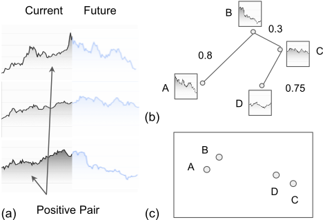
Contrastive learning [Chen et al., 2020] is a method used to enhance neural networks' ability to create strong representations by exposing them to perspectives that differ from the main task. In the context of PM, this is useful because the policy used to make investment decisions relies on the representations extracted from the data. To this end, it is beneficial to group together representations that are highly correlated, as it's possible that one asset may serve as a leading indicator of another asset in the financial market. When two assets, represented by (xit1 , xjt2 ), can assist each other in predicting future price trends, they are considered positive pairs. However, if this is not the case, the pair is considered negative. Figure 1 illustrates this idea. Note that the pairs can come from different assets and different time periods, as these relationships can occur at any time and place. For simplicity, we will omit the subscript t (i.e., xit → xi ) in the following paragraphs.
Our policy network includes an encoder f at the front that encodes an external state xi into a representation zi (i.e., zi = f(xi )). We find a corresponding state xj for each state xi in the training batch to generate positive pairs, and apply the contrastive reward to train the encoder f . The cosine similarity of vectors u and v is defined as d(u, v) = u·v/|u||v|. For each positive pair (xi , xj ) in a training batch B, we maximize the following reward:
where I[k̸=i] ∈ 0, 1 is an indicator function that returns 1 only if k ̸= i, and τ is a temperature parameter. Let P be the set of positive pairs. The total contrastive reward is given by RC = ∑i,j∈P RC (zi , zj ).
4.1 Positive Pair Matching by Forecasting.
We determine that asset states are positive pairs if they can help predict each other's future price movements. To do this, we utilize neural relational inference (NRI) [Kipf et al., 2018] to identify positive and negative pairs of asset states. NRI is a graph neural network (GNN) that is trained in an unsupervised manner to discover relationships between entities. Its structure is based on a variational autoencoder (VAE). The encoder learns the relationships from historical asset prices, and the decoder predicts future price movement trajectories. Unlike traditional VAE variants, which analyze each asset state individually, NRI takes into account all asset states in a batch when forecasting future trends.
Encoder. The encoder of NRI is a fully connected GNN as the relationships between assets are not known in advance. The network exchanges features between nodes and edges to learn the relationships. Let Φe and Φv be fully connected layers that transform features from edges to nodes and from nodes to edges, respectively. The process can be described as follows:
where hiℓ and hi,j ℓ are the representations of node i and edge {i, j} at the ℓ layer, respectively, and hi0 = xi is the input feature. The encoder uses message passing to learn the distribution of posterior relation probability:
where x = (x0 , x1 , ..., xn ) is the set of assets states. Φenc is the GNN encoder, and qϕ(ψ|x) is a categorical distribution. The relationships between nodes i and j, represented by ψi,j ∈ ψ, are learned during training, with values of ψi,j close to 1 and 0 indicating strong and weak correlations, respectively. Additionally, the sum of ψi,j for each node i over j must equal 1. Since qϕ(ψ|x) is a discrete distribution, we utilize the method proposed in [Maddison et al., 2017] to sample from a continuous approximation for updating network parameters through backpropagation. This is done by drawing samples of the form
where g is an i.i.d vector sampled from the Gumbel (0,1) distribution, and ν is a parameter used to control the smoothness of the approximation.
Decoder. The decoder predicts future price movements based on assets' current state and their relationships. That is, pθ(xt+1|xt, ψ). The decoder's architecture is similar to the encoder but in the opposite order. As a VAE, the objective is to maximize the evidence lower bound:
where the prior pθ(ψ) is a uniform categorical distribution. We also let the decoder predict multiple steps of future prices to avoid the degeneration problem because price movements can be small within a short period.
Our goal in training the NRI is to have it learn the connections between the states of assets. In practice, during the training process, we consider a pair of states (xi , xj ) to be positive if the value of ψi,j is the highest for state xi . To improve the agents' ability to create strong representations, we maximize the contrastive reward, as described in Equation 6. The representations of correlated states should be close, while the representations of uncorrelated states should be distinct.
5 Reward Smoothing
Maximizing the reward RT requires maximizing µtat · yt at each time period t. However, focusing solely on immediate returns can lead to overfitting to the training data as price movements are unpredictable. As the states of consecutive periods are similar (differing only by one period), we smooth the reward to encourage the RL agents to take similar actions in consecutive periods. We use the variable F to represent the number of future time steps used for smoothing. Along with maximizing RT , the RL agents must also maximize
It deserves noting that time-continuous batches are commonly used in network training for time series applications, which implies smoothing in the temporal dimension. However, this method and our reward smoothing are entirely different. Using samples in a batch allows the agent to trade independently at each period, and the weighting of assets in consecutive periods can be distinct. In contrast, our reward smoothing encourages the agent to take an action that will earn profits over multiple future periods. The actions taken in consecutive periods are not independent and are intended to achieve similar profits.
6 Deterministic Policy Gradient
We employ a policy gradient method to address the PM problem. The entire state-action-reward trajectory for a T period investment is represented by the sequence s1, a1, r1, ..., sT , aT , rT . At every time step t, the agent π decides the allocation weight for each asset based on the current state st using the equation
where φ indicates the network parameters. The goal is to maximize the final portfolio value RT after multiple trading steps. To help the agent learn effective strategies, two additional objectives were also employed: earning smoothed rewards sRT and extracting robust representations from asset states RC for agents to make decisions. This is done because using multiple objectives, also known as multi-task learning, has been shown to be effective for the main task in various applications [Ruder, 2017]. The overall reward for the agent π is defined as
where α is the weight that balances the rewards RT and sRT , and β is a weight that adjusts the strength of contrastive learning. Ideally, α could be a constant. However, since RT reflects the actual portfolio value, we only use sRT as a guide. Specifically, we set α = exp(-RT ), which is based on the log-portfolio value RT . The weight is high when the agent earns little or negative returns, and the weight is low otherwise. We do not adjust α based on the training iteration as it is difficult to know when the agents have learned to earn longterm rewards. This strategy also prevents the agents from overfitting to noisy rewards because low RT strengthens sRT during training. The value of α will remain high at the end of training if the reward at the next period is unpredictable.
6.1 Implementation Details
Policy. The agent's input is a state st = ⟨xt,wt⟩, which is composed of historical asset prices and the assets' weights. The external state xt contains the closing, high, and low prices of the past k time steps (k = 31). To preprocess the data, the asset prices are normalized by dividing the price of the previous period and subtracting a constant 1. Given that the future price movements of assets could be linked to their history, convolutional layers are used to extract the representation of each asset zit = f(xit ). All asset representations are concatenated and passed through another set of convolutional layers represented by g(·), which takes the concatenated zit and the assets' weights wt and outputs an action:
where z0t is a bias term and zt is the concatenated representation of all assets. The policy, denoted by π, is a composite function g ◦ f. The network architecture is illustrated in the supplemental material (Figure ??). The AdamW optimizer [Loshchilov and Hutter, 2017] is used to train the network, the discount factor γ is set to 1, the length of reward smoothing F (Equation 12) is set to 5, and the temperature τ is set to 0.05 (Equation 6). The learning rate is set to 0.0001/0.00015 and the batch size is set to 300/500 for the U.S. stock/cryptocurrency market, respectively.
The agents are trained using online learning. To begin, the policy π is trained on the training set. During back-testing, the policy continues to update by incorporating new samples after they have been evaluated. Specifically, after the agent places an order at time t and the state st+1 is observed, the state st-F and the corresponding reward are added to the training set. F is the window used for reward smoothing. We use a geometrically distributed probability function to sample data for training:
where γ ∈ (0, 1) is used to control the importance of recent states, T and nb are the lengths of the entire training data set and a single batch, respectively, and t is the time of the sample. The value of γ is set to 5e-5 for the cryptocurrency market and 5e - 4 for the U.S. stock market.
NRI. The encoder and decoder networks of theNRI are two fully connected layers with 32 hidden units and ELU activation functions. The learning rate is set to 0.00015 for the cryptocurrency market and 0.0001 for the U.S. stock market, and the temperature ν is set to 0.5. The policy and the NRI are trained simultaneously using the same batch of samples. As the price trends of consecutive states are often similar, to avoid bias, we shuffle the asset states in each batch and partition the states into groups for contrastive learning. The NRI is trained to learn the relationships of sample states within each group rather than the entire batch. In our implementation, the policy batch size is 500, with each sample containing n assets (i.e., the policy considers n/all assets at a time when trading). We set the NRI graph to contain 25 nodes, and divide the asset states into 20n groups. Since we find the closest asset state j for each state i, this means that each NRI graph forms 25 positive pairs and 25 × 24 negative pairs, and the NRI batch size is 20n.
7 Evaluations
In order to evaluate our model, we compared it to previous methods in the U.S. stock market and cryptocurrency market.
7.1 Baselines
We compared our method to a variety of traditional and DRL methods. These traditional methods include Buy and Hold, uniform constant rebalanced portfolio (UCRP) [Cover, 2011], on-line moving average reversion (OLMAR) [Li and Hoi, 2012], and weighted moving average mean reversion (WMAMR) [Gao and Zhang, 2013]. The DRL methods include deep portfolio management (DPM) [Jiang et al., 2017] and the state-augmented RL (SARL) [Ye et al., 2020]. Additional information about these baselines can be found in the supplemental material or in the corresponding papers.
The implementations of UCRP, OLMAR, WMAMR, and DPM were obtained from Jiang et al.'s [2017] GitHub page 1 , we have implemented the Buy and Hold and SARL method as the former is a simple method and the latter's implementation is not available. We have taken care to ensure that the comparison is fair by closely following the details of SARL's paper. In addition, for the two DRL baselines, DPM and SARL, we experimented with deeper policy networks, which have the same architecture as our model, and denoted them by DPM v2 and SARL v2, respectively, in the comparison.
1 https://github.com/ZhengyaoJiang/PGPortfolio
7.2 EvaluationMetrics
The performance of the investment strategies was compared using standard evaluation metrics, including portfolio value, Sharpe ratio, and maximum drawdown. As these metrics are not flawless, it's important to take into account all of them when evaluating the methods. More information about these metrics can be found in the supplemental material.
7.3 Data and Experiment Setup
We followed the experimental setup from previous studies [Jiang et al., 2017; Ye et al., 2020] in our experiments. Specifically, we set the transaction fees cs = cp = 0.25% for both buying and selling assets, which is the highest rate on Poloniex. The agents trade at the opening and receive a reward at the closing of each period. We compared our method to the baselines on the U.S. stock market and cryptocurrency market. The data was obtained from the Yahoo Finance Application Programming Interface (API) and the Poloniex's official API, respectively. We selected assets with high trading volumes for the experiment. For the U.S. stock market, we collected daily frequency data for the nine highest trading stocks (GOOG, NVDA, AMZN, AMD, QCOM, INTC, MSFT, AAPL, and BIDU). In the cryptocurrency market, we collected half-hour frequency data for the ten highest trading cryptocurrencies (ETH, LTC, XRP, USDT, ETC, DASH, XMR, XEM, GNT, ZEC, and BTC is the cash).
We carried out experiments on the U.S. stock market and the cryptocurrency market to evaluate our model. For the U.S. stock market, the data covered the dates from 2006-1020 to 2013-11-20, from 2003-06-20 to 2011-08-20, and from 2001-02-20 to 2009-05-20 respectively. The data collected in these three periods were separated chronologically and the last year's data were used for testing. In the cryptocurrency market, we selected the dates from 2015-12-30 to 2018-0131, from 2016-03-05 to 2018-02-28, and from 2016-04-05 to 2018-03-31. In this experiment, the last two months of data were used for testing. The testing periods have different lengths because of the different data frequencies. In the U.S. stock market, the agents trade once per day, while in the cryptocurrency market, they trade once per 30 minutes. It is worth noting that the overall trends of the testing periods were an increase, no change, and a decrease, respectively. This is because we were interested in the model's performance under different market conditions.
The performance of RL agents can be greatly impacted by their initialization. To account for this, we trained agents from 8 different random seeds and reported their mean portfolio values. We also conducted an ablation study to evaluate the effectiveness of the proposed contrastive reward, reward smoothing, and their combination. Furthermore, to demonstrate the ability of our method in generating effective positive
| Method | Increase | No change | Decrease | ||||||
|---|---|---|---|---|---|---|---|---|---|
| PV ↑ | SR ↑ | MDD ↓ | PV ↑ | SR ↑ | MDD ↓ | PV ↑ | SR ↑ | MDD ↓ | |
| Buy & Hold | 1.39 | 2.13 | 0.06 | 1.14 | 0.62 | 0.17 | 0.87 | -0.05 | 0.54 |
| Mean-Variance | 0.92 | -0.15 | 0.18 | 1.07 | 0.34 | 0.23 | 0.31 | -1.14 | 0.83 |
| UCRP | 1.40 | 2.41 | 0.05 | 1.14 | 0.63 | 0.16 | 0.95 | 0.13 | 0.54 |
| OLMAR | 0.72 | -0.04 | 0.49 | 0.53 | -0.07 | 0.53 | 0.66 | -0.003 | 0.74 |
| WMAMR | 1.18 | 0.70 | 0.17 | 0.40 | -1.96 | 0.63 | 0.57 | -0.30 | 0.78 |
| DPM | 1.23 ± 0.20 | 0.75 | 0.20 | 1.16 ± 0.03 | 0.51 | 0.21 | 0.75 ± 0.09 | -0.27 | 0.62 |
| DPM v2 | 1.38 ± 0.10 | 1.21 | 0.29 | 1.26 ± 0.12 | 0.67 | 0.26 | 1.05 ± 0.04 | 0.26 | 0.60 |
| SARL | 1.13 ±0.23 | 0.47 | 0.27 | 1.13 ± 0.05 | 0.42 | 0.22 | 0.72 ± 0.12 | -0.24 | 0.64 |
| SARL v2 | 1.37 ± 0.39 | 1.01 | 0.32 | 1.12 ± 0.04 | 0.41 | 0.20 | 0.98 ± 0.29 | 0.19 | 0.70 |
| Ours (TS2VEC) | 1.25 ± 0.20 | 0.83 | 0.31 | 1.45 ± 0.18 | 0.97 | 0.23 | 1.14 ± 0.44 | 0.29 | 0.61 |
| Ours (TS2VEC+sRT) | 1.38 ± 0.23 | 1.14 | 0.30 | 1.25 ± 0.21 | 0.57 | 0.26 | 0.97 ± 0.14 | 0.21 | 0.64 |
| Ours (PPM) | 1.50 ± 0.09 | 1.59 | 0.21 | 1.54 ± 0.15 | 1.09 | 0.23 | 1.12 ± 0.27 | 0.32 | 0.64 |
| Ours (sRT) | 1.62 ± 0.11 | 1.63 | 0.23 | 1.26 ± 0.14 | 0.91 | 0.23 | 1.25 ± 0.42 | 0.47 | 0.60 |
| Ours (PPM+sRT) | 1.69 ± 0.09 | 1.61 | 0.25 | 1.35 ± 0.18 | 0.76 | 0.25 | 1.17 ± 0.37 | 0.39 | 0.59 |
Cryptocurrency Market
| Method | Increase | No change | Decrease | ||||||
|---|---|---|---|---|---|---|---|---|---|
| PV ↑ | SR ↑ | MDD ↓ | PV ↑ | SR ↑ | MDD ↓ | PV ↑ | SR ↑ | MDD ↓ | |
| Buy & Hold | 2.27 | 4.31 | 0.35 | 1.06 | 0.83 | 0.20 | 0.77 | -3.51 | 0.33 |
| Mean-Variance | 0.16 | -4.00 | 0.84 | 0.06 | -12.38 | 0.94 | 0.04 | -20.55 | 0.96 |
| UCRP | 2.28 | 5.03 | 0.36 | 1.16 | 1.67 | 0.19 | 0.79 | -2.98 | 0.32 |
| OLMAR | 0.08 | -0.031 | 0.915 | 0.30 | -0.019 | 0.807 | 0.53 | -0.013 | 0.757 |
| WMAMR | 0.59 | -0.11 | 0.67 | 0.49 | -1.18 | 0.59 | 0.35 | -3.89 | 0.71 |
| DPM | 6.03 ± 1.39 | 6.25 | 0.28 | 9.60 ± 2.23 | 7.84 | 0.30 | 22.54 ± 5.04 | 12.52 | 0.26 |
| DPM v2 | 9.00 ± 1.79 | 6.73 | 0.31 | 19.73 ± 3.61 | 9.87 | 0.28 | 56.92 ± 9.58 | 15.49 | 0.21 |
| SARL | 8.00 ± 1.97 | 6.79 | 0.27 | 12.03 ± 2.74 | 8.42 | 0.27 | 21.47 ± 3.84 | 12.97 | 0.26 |
| SARL v2 | 10.36 ± 1.61 | 7.38 | 0.26 | 22.28 ± 5.56 | 10.22 | 0.27 | 47.80 ± 9.65 | 14.82 | 0.21 |
| Ours (TS2VEC) | 14.87 ± 5.51 | 7.78 | 0.27 | 144.57 ± 37.77 | 17.12 | 0.28 | 1287.1 ± 348.1 | 31.78 | 0.18 |
| Ours (TS2VEC+sRT) | 18.43 ± 5.53 | 7.83 | 0.29 | 129.73 ± 32.18 | 16.14 | 0.29 | 1292.2 ± 150.1 | 30.03 | 0.20 |
| Ours (PPM) | 11.56 ± 2.70 | 7.46 | 0.30 | 130.77 ± 27.86 | 16.73 | 0.30 | 1374.8 ± 253.3 | 32.15 | 0.19 |
| Ours (sRT) | 15.07 ± 10.56 | 7.28 | 0.30 | 145.00 ± 41.73 | 16.50 | 0.30 | 1455.9 ± 284.8 | 31.58 | 0.19 |
| Ours (PPM+sRT) | 21.50 ± 10.10 | 8.05 | 0.29 | 166.69 ± 37.42 | 17.00 | 0.29 | 1356.1 ± 470.8 | 31.38 | 0.17 |
and negative pairs of time series data for contrastive learning, we compared it to the latest time series data augmentation approach, TS2VEC [Yue et al., 2021], and evaluated their performances. The role of TS2VEC is similar to our positive pair matching and its goal is to assist RL agents in learning robust representations.
7.4 Results of the Comparison
Table 1 shows the results of the experiments comparing various baselines. Notably, Buy & Hold strategy's portfolio values align with market trends, as it evenly distributes capital across assets initially and sells them all at the end of the period. The traditional PM methods underperformed the DRL methods by a significant margin, consistent with findings from recent studies [Sutton and Barto, 2018].
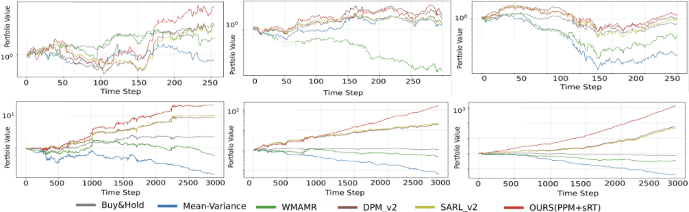
DRL methods showed promising performance as the agents were trained to maximize returns over multiple steps. As seen in Figure 2, DRL methods generally performed better than traditional techniques except for a specific period when the overall price trend is increasing in the U.S. stock market. However, DRL methods did not always guarantee low risk as the values of SR and MDD were worse than traditional methods in certain markets, which aligns with the understanding that high returns come with high risks. Additionally, since all DRL agents in this study were trained solely to maximize portfolio values, it is not surprising that they adopted high-risk strategies. Compared to DPM and SARL, our method achieved not only high portfolio values but also high Sharpe ratios. The advantage was gained through contrastive learning, reward smoothing, and a deeper policy network. As shown in Table 1, DPM v2 and SARL v2 consistently performed better than DPM and SARL in all market conditions. This could be attributed to the deeper network providing better generalization as demonstrated in other experiments [Yang et al., 2020; Neyshabur et al., 2018]. However, even with the deeper policy network, our method still outperformed DPM v2 and SARL v2 due to the added benefits of contrastive learning and reward smoothing.
Our model exhibited strong performance in the cryptocurrency market as compared to the U.S. stock market. This can be attributed to the fact that our agents executed significantly more trades in the cryptocurrency market, leading to compound interest and higher returns. Furthermore, the model achieved positive returns even when the overall price trend in a cryptocurrency market is downward. This was made possible by a significant increase in the USDT/BTC ratio, as our RL agents strategically allocated a substantial portion of their capital to this investment.
7.5 Results of the Ablation Study
The results of the ablation study, as seen in Table 1, suggest that both the contrastive reward and reward smoothing had a positive impact. Specifically, the combination of our smoothed reward and contrastive learning (PPM+sRT) performed the best when the overall price trend is downward, as the smoothed reward can act as a regularization and lead to more conservative strategies. Overall, it can be seen that a combination of the two training strategies is beneficial. The high portfolio values and Sharpe ratios observed in markets, when comparing DPM v2, Ours(TS2VEC+sRT), and Ours(PPM+sRT), which share the same network architecture, demonstrate the effectiveness of these two training strategies. While the TS2VEC [Yue et al., 2021] approach showed some benefits, the performance of TS2VEC+sRT was not as good as PPM+sRT. This could be due to the different ways in which positive pairs are defined, with our PPM expecting asset states to be highly-related in future price movements, while TS2VEC uses mask augmentation. As PPM learned representations contain future forecasting, the task is more compatible with earning smoothed rewards, thus allowing the agent to learn better trading strategies by tackling the correlated sub-tasks [Crawshaw, 2020].
7.6 Significance of the Results
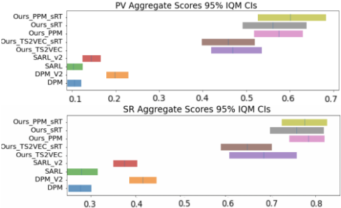
While financial markets are highly uncertain, it is impractical to expect a strategy consistently outperforms others throughout all periods. We thus employed the interquartile mean (IQM) to evaluate the statistical significance of the results. Figure 3 presents the aggregated outcomes across the U.S. stock and cryptocurrency markets. The 95% confidence intervals (i.e., the bars) show that PPM+sRT substantially surpasses the baselines. Details will be provided in Appendix.
7.7 Limitations
While our RL model demonstrated strong performance when evaluated on historical data, this does not necessarily guarantee success in a live trading scenario. Besides, financial markets are inherently uncertain and subject to change. Therefore, combining contrastive learning and reward smoothing may not always result in the highest returns. We also found that the results in terms of Sharpe ratio and maximum drawdown in Table 1 indicate that our method does not necessarily balance both high returns and low volatility.
8 Conclusions
We developed a DRL based method for training agents to trade in financial markets with the goal of maximizing cumulative returns. Our approach includes the use of contrastive reward and reward smoothing to assist agents in learning robust representations in the face of uncertain future price movements. We evaluated our method against several baselines on both the U.S. stock market and the cryptocurrency market and found that it performed well in these experiments. The ablation study also supported the effectiveness of our method. While our method showed promising results, there are still limitations. We will address this in future work.
Acknowledgments
We thank the reviewers for their constructive comments. This work was supported by E.SUN Bank and the National Science and Technology Council, Taiwan (111-2221-E-A49 - 129 -MY3 and 111-2634-F-A49 -013 -).
@inproceedings{ijcai2023p441,
  title     = {Contrastive Learning and Reward Smoothing for Deep Portfolio Management},
  author    = {Lien, Yun-Hsuan and Li, Yuan-Kui and Wang, Yu-Shuen},
  booktitle = {Proceedings of the Thirty-Second International Joint Conference on
               Artificial Intelligence, {IJCAI-23}},
  publisher = {International Joint Conferences on Artificial Intelligence Organization},
  editor    = {Edith Elkind},
  pages     = {3966--3974},
  year      = {2023},
  month     = {8},
  note      = {Main Track},
  doi       = {10.24963/ijcai.2023/441},
  url       = {https://doi.org/10.24963/ijcai.2023/441},
}
TY - CPAPER TI - Contrastive Learning and Reward Smoothing for Deep Portfolio Management AU - Lien, Yun-Hsuan AU - Li, Yuan-Kui AU - Wang, Yu-Shuen T2 - Proceedings of the Thirty-Second International Joint Conference on Artificial Intelligence, IJCAI-23 PB - International Joint Conferences on Artificial Intelligence Organization PY - 2023 SP - 3966 EP - 3974 DO - 10.24963/ijcai.2023/441 UR - https://doi.org/10.24963/ijcai.2023/441 ER -Copied
Machine-readable versions of this paper, for tools and AI agents:





