
RAIN: RegulArization on Input and Network for Black-Box Domain Adaptation
Proceedings of the Thirty-Second International Joint Conference on Artificial Intelligence. Main Track. Pages 4118-4126.
https://doi.org/10.24963/ijcai.2023/458
Keywords
- Machine Learning: ML: Multi-task and transfer learning
- Computer Vision: CV: Transfer, low-shot, semi- and un- supervised learning
Abstract
Source-Free domain adaptation transits the source-trained model towards target domain without exposing the source data, trying to dispel these concerns about data privacy and security. However, this paradigm is still at risk of data leakage due to adversarial attacks on the source model. Hence, the Black-Box setting only allows to use the outputs of source model, but still suffers from overfitting on the source domain more severely due to source model's unseen weights. In this paper, we propose a novel approach named RAIN (RegulArization on Input and Network) for Black-Box domain adaptation from both input-level and network-level regularization. For the input-level, we design a new data augmentation technique as Phase MixUp, which highlights task-relevant objects in the interpolations, thus enhancing input-level regularization and class consistency for target models. For network-level, we develop a Subnetwork Distillation mechanism to transfer knowledge from the target subnetwork to the full target network via knowledge distillation, which thus alleviates overfitting on the source domain by learning diverse target representations. Extensive experiments show that our method achieves state-of-the-art performance on several cross-domain benchmarks under both single- and multi-source black-box domain adaptation.
- [Ahmed et al., 2021] Sk Miraj Ahmed, Dripta S Raychaud- huri, Sujoy Paul, Samet Oymak, and Amit K Roy- Chowdhury. Unsupervised multi-source domain adapta- tion without access to source data. In Proceedings of the IEEE/CVF Conference on Computer Vision and Pattern Recognition, pages 10103-10112, 2021.
- [Chen et al., 2022] Dian Chen, Dequan Wang, Trevor Dar- rell, and Sayna Ebrahimi. Contrastive test-time adaptation. arXiv preprint arXiv:2204.10377, 2022.
- [Deng et al., 2021] Wanxia Deng, Qing Liao, Lingjun Zhao, Deke Guo, Gangyao Kuang, Dewen Hu, and Li Liu. Joint clustering and discriminative feature alignment for unsu- pervised domain adaptation. IEEE Transactions on Image Processing, pages 7842-7855, 2021.
- [Dosovitskiy et al., 2020] Alexey Dosovitskiy, Lucas Beyer, Alexander Kolesnikov, Dirk Weissenborn, Xiaohua Zhai, Thomas Unterthiner, Mostafa Dehghani, Matthias Min- derer, Georg Heigold, Sylvain Gelly, et al. An image is worth 16x16 words: Transformers for image recognition at scale. arXiv preprint arXiv:2010.11929, 2020.
- [Ganin and Lempitsky, 2015] Yaroslav Ganin and Victor Lempitsky. Unsupervised domain adaptation by backprop- agation. In International Conference on Machine Learn- ing, pages 1180-1189, 2015.
- [Goodfellow et al., 2014] Ian Goodfellow, Jean Pouget- Abadie, Mehdi Mirza, Bing Xu, David Warde-Farley, Sherjil Ozair, Aaron Courville, and Yoshua Bengio. Gen- erative adversarial nets. Advances in Neural Information Processing Systems, 27, 2014.
- [He et al., 2016] Kaiming He, Xiangyu Zhang, Shaoqing Ren, and Jian Sun. Deep residual learning for image recognition. In Proceedings of the IEEE Conference on Computer Vision and Pattern Recognition, pages 770-778, 2016.
- [Hinton et al., 2015] Geoffrey Hinton, Oriol Vinyals, and Jeff Dean. Distilling the knowledge in a neural network. STAT, 2015.
- [Hou and Zheng, 2021] Yunzhong Hou and Liang Zheng. Visualizing adapted knowledge in domain transfer. In Pro- ceedings of the IEEE/CVF Conference on Computer Vision and Pattern Recognition, pages 13824-13833, 2021.
- [Kurmi et al., 2021] Vinod K Kurmi, Venkatesh K Subrama- nian, Vinay P Namboodiri, , and . Domain impression: A source data free domain adaptation method. In Proceed- ings of the IEEE/CVF Winter Conference on Applications of Computer Vision, pages 615-625, 2021.
- [Li et al., 2020] Rui Li, Qianfen Jiao, Wenming Cao, Hau- San Wong, and Si Wu. Model adaptation: Unsuper- vised domain adaptation without source data. In 2020 IEEE/CVF Conference on Computer Vision and Pattern Recognition (CVPR), pages 9638-9647, 2020.
- [Liang et al., 2020] Jian Liang, Dapeng Hu, and Jiashi Feng. Do we really need to access the source data? source hypothesis transfer for unsupervised domain adaptation. In International Conference on Machine Learning, pages 6028-6039. PMLR, 2020.
- [Liang et al., 2022] Jian Liang, Dapeng Hu, Ran He, and Ji- ashi Feng. Dine: Domain adaptation from single and mul- tiple black-box predictors. Proceedings of the IEEE/CVF Conference on Computer Vision and Pattern Recognition (CVPR), pages 8003-8013, June 2022.
- [Liu et al., 2021] Quande Liu, Cheng Chen, Jing Qin, Qi Dou, and Pheng-Ann Heng. Feddg: Federated do- main generalization on medical image segmentation via episodic learning in continuous frequency space. In Pro- ceedings of the IEEE/CVF Conference on Computer Vision and Pattern Recognition, pages 1013-1023, 2021.
- [Long et al., 2015] Mingsheng Long, Yue Cao, Jianmin Wang, and Michael Jordan. Learning transferable features with deep adaptation networks. In International Confer- ence on Machine Learning, pages 97-105, 2015.
- [Long et al., 2017] Mingsheng Long, Han Zhu, Jianmin Wang, and Michael I Jordan. Deep transfer learning with joint adaptation networks. In International conference on machine learning, pages 2208-2217. PMLR, 2017.
- [Muller et al., 2019] Rafael Muller, Simon Kornblith, and Geoffrey E Hinton. When does label smoothing help? Ad- vances in Neural Information Processing Systems, 2019.
- [Paszke et al., 2019] Adam Paszke, Sam Gross, Francisco Massa, Adam Lerer, James Bradbury, Gregory Chanan, Trevor Killeen, Zeming Lin, Natalia Gimelshein, Luca Antiga, et al. Pytorch: An imperative style, high- performance deep learning library. Advances in Neural Information Processing Systems, 2019.
- [Peng et al., 2017] Xingchao Peng, Ben Usman, Neela Kaushik, Judy Hoffman, Dequan Wang, and Kate Saenko. Visda: The visual domain adaptation challenge. arXiv preprint arXiv:1710.06924, 2017.
- [Ruder, 2016] Sebastian Ruder. An overview of gradi- ent descent optimization algorithms. arXiv preprint arXiv:1609.04747, 2016.
- [Saenko et al., 2010] Kate Saenko, Brian Kulis, Mario Fritz, and Trevor Darrell. Adapting visual category models to new domains. In European Conference on Computer Vi- sion, pages 213-226, 2010.
- [Saito et al., 2018] Kuniaki Saito, Kohei Watanabe, Yoshi- taka Ushiku, and Tatsuya Harada. Maximum classifier discrepancy for unsupervised domain adaptation. In Pro- ceedings of the IEEE Conference on Computer Vision and Pattern Recognition, pages 3723-3732, 2018.
- [Shorten and Khoshgoftaar, 2019] Connor Shorten and Taghi M Khoshgoftaar. A survey on image data augmen- tation for deep learning. Journal of Big Data, 6(1):1-48, 2019.
- [Tang et al., 2020] Hui Tang, Ke Chen, and Kui Jia. Un- supervised domain adaptation via structurally regularized deep clustering. In Proceedings of the IEEE/CVF Confer- ence on Computer Vision and Pattern Recognition, pages 8725-8735, 2020.
- [Tzeng et al., 2014] Eric Tzeng, Judy Hoffman, Ning Zhang, Kate Saenko, and Trevor Darrell. Deep domain confu- sion: Maximizing for domain invariance. arXiv preprint arXiv:1412.3474, 2014.
- [Van der Maaten and Hinton, 2008] Laurens Van der Maaten and Geoffrey Hinton. Visualizing data using t-sne. Journal of machine learning research, 9(11), 2008.
- [Venkateswara et al., 2017] Hemanth Venkateswara, Jose Eusebio, Shayok Chakraborty, and Sethuraman Pan- chanathan. Deep hashing network for unsupervised do- main adaptation. In Proceedings of the IEEE Conference on Computer Vision and Pattern Recognition, pages 5018- 5027, 2017.
- [Wang and Deng, 2018] Mei Wang and Weihong Deng. Deep visual domain adaptation: A survey. Neurocomput- ing, 312:135-153, 2018.
- [Wang et al., 2018] Tongzhou Wang, Jun-Yan Zhu, Antonio Torralba, and Alexei A Efros. Dataset distillation. arXiv preprint arXiv:1811.10959, 2018.
- [Wu et al., 2020] Yuan Wu, Diana Inkpen, and Ahmed El- Roby. Dual mixup regularized learning for adversarial do- main adaptation. In European Conference on Computer Vision, pages 540-555. Springer, 2020.
- [Xia et al., 2021] Haifeng Xia, Handong Zhao, and Zheng- ming Ding. Adaptive adversarial network for source-free domain adaptation. In Proceedings of the IEEE/CVF In- ternational Conference on Computer Vision, pages 9010- 9019, 2021.
- [Yang and Soatto, 2020] Yanchao Yang and Stefano Soatto. Fda: Fourier domain adaptation for semantic segmenta- tion. In Proceedings of the IEEE/CVF Conference on Computer Vision and Pattern Recognition, pages 4085- 4095, 2020.
- [Yin et al., 2020] Hongxu Yin, Pavlo Molchanov, Jose M Al- varez, Zhizhong Li, Arun Mallya, Derek Hoiem, Niraj K Jha, and Jan Kautz. Dreaming to distill: Data-free knowl- edge transfer via deepinversion. In Proceedings of the IEEE/CVF Conference on Computer Vision and Pattern Recognition, pages 8715-8724, 2020.
- [YM. et al., 2020] Asano YM., Rupprecht C., and Vedaldi A. Self-labelling via simultaneous clustering and represen- tation learning. In International Conference on Learning Representations, 2020.
- [Yun et al., 2019] Sangdoo Yun, Dongyoon Han, Seong Joon Oh, Sanghyuk Chun, Junsuk Choe, and Youngjoon Yoo. Cutmix: Regularization strategy to train strong classifiers with localizable features. In Proceedings of the IEEE/CVF international conference on computer vision, pages 6023- 6032, 2019.
- [Zhang et al., 2018] Hongyi Zhang, Moustapha Cisse, Yann N. Dauphin, and David Lopez-Paz. mixup: Beyond empirical risk minimization. In International Conference on Learning Representations, 2018.
- [Zhang et al., 2021] Haojian Zhang, Yabin Zhang, Kui Jia, and Lei Zhang. Unsupervised domain adaptation of black- box source models. arXiv preprint arXiv:2101.02839, 2021.
References were extracted automatically from the PDF and may contain errors.
Full text extracted automatically from the PDF; figures, tables and equations may differ. The PDF is the version of record.
1 Introduction
Domain adaptation [Wang and Deng, 2018] is proposed to transfer knowledge from the labeled training data that form the source domain to the unlabeled test data that form the target domain. Owing to the concerns about data privacy and security, a new setting -Source-Free domain adaptation [Liang et al., 2020]- emerges, where source data are completely unavailable when adapting to the target. Even so, there are still potential risks if the source models are visible. Some works like dataset distillation [Wang et al., 2018] and DeepInversion [Yin et al., 2020] may recover data from the model through adversarial attacks. In such a case, Black-Box domain adaptation [Zhang et al., 2021] is proposed to consider the source models are completely unseen and only model outputs are accessible for target adaptation, which is a more strict version of Source-Free domain adaptation.
Due to the limited access to the source model, the only way we obtain source information is by doing knowledge distilling between the source model and the target model. In the original Source-Free setting, we can alleviate domain shifts by updating the source model gradually, keeping the transferrable parameters while replacing the untransferrable ones. However, in the Black-box scenario, only the source model's outputs are exposed, i.e., the source information cannot be disentangled as target-relevant and target-irrelevant parts as Source-Free does. The overfitting on the source domain in Black-Box is much stronger than that in Source-free, which greatly undermines the target models' performance. [Liang et al., 2022] observes this problem and uses conventional MixUp [Zhang et al., 2018] as regularization for better generalization. However, there exist problems with regularization methods like MixUp or CutMix [Yun et al., 2019] because they are conducted on both input and label levels. In the target adaptation process, we do not have accurate labels but the pseudo labels as substitutes and the linear behaviors learned from these noisy pseudo-labels due to domain shifts could have negative impacts on the generalization and degrade the model's performance (details in Table 4).
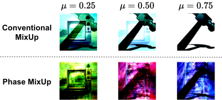
Based on the discussions above, we develop a new and effective data augmentation method for domain adaptation named Phase MixUp, which regularizes ML model training only from the input aspect. Apart from inhibiting potential noises from pseudo-labels, our Phase MixUp can highlight task-relevant objects and avoid negative impacts from background information as well. Conventional MixUp directly blends one image's pixels into another image [Wu et al., 2020; Liang et al., 2022]. But this kind of combination is too simple to highlight the objects that we want to classify, especially when the image owns complex background and style information. For example, the top of Fig. 1 shows the conventional MixUp between the "television" image and the "hammer" image. The "hammer" image has a very strong dark shadow that outweighs another object "television" when µ = 0.50. Besides, when µ = 0.75, the "television" is completely unseen. In such cases, background elements like dark shadow will have a negative impact on conventional MixUp as they distract the attention of core objects and the model tends to connect the "hammer" with the shadow instead. Frequency decomposition proves to be a useful tool to disentangle object information and background information from an image [Yang and Soatto, 2020; Liu et al., 2021], since amplitude spectra contain most background information, while phase spectra are related to object information. Therefore, we propose Phase MixUp (Fig. 2b) to capture the key objects and reduce background interference at the same time, as the bottom of Fig. 1 shows. By mixing their phase spectra, we can focus more on the two core objects "television" and "hammer" and weaken background information like the shadow. Even under a more extreme case like µ = 0.75, the "television" still exists in the mixed image of Phase MixUp. The augmented image will attend further training to enhance the target model's class consistency.
What's more, despite the fact that input- and label-level regularizations have received enough attention in domain adaptation, regularization from the network aspect is overlooked. Specifically, in the Black-Box setting, only the source model's outputs are accessible, which leads to more severe overfitting of target networks on source information. Because target networks have to learn from the outputs produced by source models without detailed calibrations on network weights as the Source-Free setting does. Therefore, a network-level regularization technique on target networks is necessary. To this end, we propose a novel method for domain adaptation called Subnetwork Distillation, which aims to regularize the full target network with the help of its subnetwork and calibrate the full target networks gradually. We slim the widths of the target network to get its subnetwork, which has a smaller scale than the full network, hence less likely overfitting to the source domain. By transferring knowledge from the target subnetwork to the full target network, the original full network captures diverse representations from the target domain with a better generalization ability.
Our contributions are summarized in three aspects:
- We propose Phase MixUp as a new input-level regularization scheme that helps the model enhance class consistency
- with more task-relevant object information, thus obtaining more robust representations for the target domain.
- We introduce a novel network-level regularization technique called Subnetwork Distillation that assists the target model to learn diverse representations and transfers knowledge from the model's partial structures to avoid overfitting on Black-Box source models.
- We conduct extensive experimental results on several benchmark datasets with both Single-Source and MultiSource settings, showing that our approach achieves stateof-the-art performance compared with the latest methods for Black-Box domain adaptation.
2 RelatedWork
Domain Adaptation. Metric-based and GAN-based approaches are the two major routes in single-source domain adaptation. The metric-based methods measure the discrepancy between the source and target domain explicitly. [Long et al., 2015] uses maximum mean discrepancy, while [Tzeng et al., 2014] applies deep domain confusion. Recent work like [Deng et al., 2021] jointly makes clustering and discrimination for alignment together with contrastive learning. The GAN-based methods originate from [Goodfellow et al., 2014] and build a min-max game for two players related to the source and target domains. [Ganin and Lempitsky, 2015] adopts domain to confuse the two players, while [Saito et al., 2018] uses classifier discrepancy as the objective, and [Tang et al., 2020] reveals that discriminative clustering on target will benefit the adaptation. However, the general domain adaptation setting needs access to source data, which raises concerns about data privacy and security, so SourceFree adaptation is proposed.
Source-Free Domain Adaptation. Based on the work of [Li et al., 2020; Liang et al., 2020], Source-Free has become the mainstream paradigm for alleviating concerns about data privacy and security in domain adaptation. There are two technique routes under the source-free setting: self-supervision and virtual source transfer. For the selfsupervised methods, [Liang et al., 2020] is the most representative one, which introduces information maximization to assist adaptation. [Xia et al., 2021] treats the problem from a discriminative perspective and adds a specific representation learning module to help the generalization, and [Chen et al., 2022] proposes the online pseudo label refinement. As for virtual source methods, most of them build GANs to generate virtual source data. [Kurmi et al., 2021] uses conditional GAN to generate new samples, while [Hou and Zheng, 2021] provides interesting visualizations for unseen knowledge and [Li et al., 2020] applies collaborative GAN to achieve better generations. But Source-Free is still at risk of data leakage due to adversarial attacks to visible model weights, and that leads to a more strict setting - Black-Box domain adaptation.
Black-Box Domain Adaptation is a subset problem of Source-Free domain adaptation and is also a very novel topic. It is more strict than Source-Free because the models trained on source will be put into a black box and only the outputs of these models can be used during model adaptation. [Zhang et al., 2021] first states this setting completely and emphasizes the purification of noisy labels in the adaptation. [Liang et al., 2022] introduces knowledge distillation to the blackbox problem, which largely improves the performance. All the details are the same as the Source-Free setting except that the source model strictly follows the Black-Box rule as its weights are completely invisible while outputs are accessible.
3 Methodology
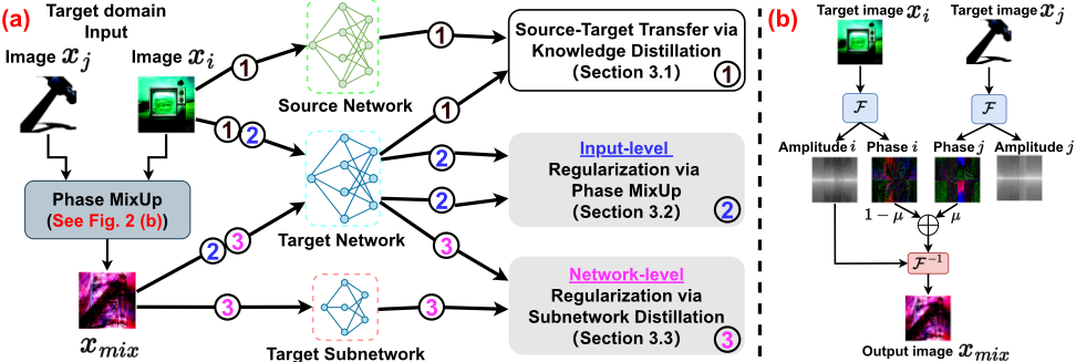
Our proposed method RAIN tackles the Black-Box domain adaptation from the perspective of regularization (both inputlevel and network-level). The overall framework is presented in Fig. 2a. In the following subsections, we elaborate on the key components of the framework.
3.1 Preliminary
For a typical domain adaptation problem, we have a source domain dataset S = {(xsi , ys i )}ns i=1 with ns labeled samples. The target domain dataset T = {xti }nt i=1 includes nt unlabeled samples, which shares the same label space D = {1, 2, · · · ,K} with source but lie in different distributions, where K is the number of classes. The goal of domain adaptation is to seek the best target model ft with the help of source model as fs.
For the Black-Box paradigm, the learning starts with the supervised learning on source as Ls = -E(xsi ,ys i )∈S ∑k∈D ls i log fs(xsi ) with label smoothing [Muller et al., 2019]: ls i = α/K + (1 - α)ys i , where α is smoothing parameter empirically set to 0.1. Moreover, the source model's details are completely unseen except for the model's outputs. In this case, knowledge distillation [Hinton et al., 2015] is applied to transfer from source to target:
where DKL(·) denotes Kullback-Leibler (KL) Divergence and ˆ yt i is the pseudo-label. Now we explain how to obtain ˆ yt i . Assume that q = arg max fs(xti ), then we deduce the smooth pseudo label lt i = α′ /K + (1 - α′ )q, where α′ is smoothing parameter empirically set to 0.1. Based on this, the pseudo label ˆ yt i can be represented as ˆ yt i = ηlt i + (1 - η)ft(xti ), where η is a momentum hyperparameter set as 0.6.
3.2 Enhancing Input Regularization via Phase MixUp
Conventional MixUp is a very popular input- and label-level regularization technique in domain adaptation [Wu et al., 2020; Liang et al., 2022], whose goal is to enhance class-wise consistency and linear behavior, thus helping the model learn better representations on target domain. Nevertheless, there exist noises in the pseudo-labels applied to MixUp, which are harmful to the adaptation process, and that's why we propose an input-level (only) regularization method here. Next details of the proposed Phase MixUp process are presented. We begin by introducing the standard format of the Fourier transform. Assume a target sample xti ∈ RC×H×W , where C, H and W correspond to channel numbers, height and width. We transfer it from spatial space to frequency space and then decompose its frequency spectrum as amplitude and phase:
Here we ensure the one-to-one correspondence between channels of different spaces. Here xti is a spatial image representation based on image pixel (h,w), and F t i is a frequency image representation based on frequency spectrum unit (u, v). Ati is the amplitude spectrum and P t i is the phase spectrum of the target sample xti . According to [Yang and Soatto, 2020; Liu et al., 2021], the amplitude spectrum reflects the low-level distributions like the style, and the high-level semantics like object shape is stored in the phase spectrum. Since our task here is domain adaptation for object recognition, we hope the mixup procedure focuses more on the key objects rather than the background information. Hence, we interpolate between phase spectra as:
where P t j is the phase spectrum from a randomly-selected target sample xtj as F(xtj ) = Atj exp (P t j ), and µ is sampled from a Beta distribution as Beta(0.3, 0.3). After that, the Phase MixUp augmented sample produced by inverse Fourier Transform is:
The Phase MixUp procedure is depicted in Fig. 2b. After obtaining the synthesized sample, we can enhance class consistency by comparing the outputs of the original and synthesized samples. Here ℓ1-norm is utilized to compute the Phase MixUp loss as:
Phase MixUp is different from conventional MixUp. First, our Phase MixUp is conducted on the phase spectra related to core objects, not the whole image. Moreover, conventional MixUp operates on both input- and label-level, while Phase MixUp is an input-level augmentation.
3.3 Encouraging Network Regularization via Subnetwork Distillation
During the procedure of knowledge transfer from source models to target models with knowledge distillation (Eq. 1), overfitting on source information is an obvious side effect. Especially in the Black-Box setting, only the source model's outputs are visible while the source model's weights are completely unseen. In other words, the careful calibration of the target network's weights in the Source-Free setting cannot be achieved here. Hence, it is necessary to propose a specific network-based regularization method.To this end, we propose the Subnetwork Distillation approach to domain adaptation, which utilizes the self-knowledge transfer from the target subnetwork to the full target network with distinctive knowledge. We hope this structure can assist the model to obtain more target information from diverse representations far from the support of source, thus overcoming overfitting on source. We denote the full target network's weights as Wfull and the target subnetwork as Wsub. If the complete network can be represented as Wfull = W0:1, then by slimming the network width with a ratio α ∈ (0, 1], the subnetwork can be generated as Wsub = W0:α, i.e., a subnetwork with W0:α means selecting the first α × 100% weights of each layer of the full network. Therefore, the network's output with width α is denoted as ft(xti ;W0:α). The Subnetwork Distillation objective is defined as
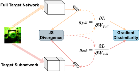
After getting these outputs from the subnetwork with smaller widths, we compare them with the original network's outputs using Jensen-Shannon (JS) divergence, shown in Fig. 3. To prevent the adverse influence on the inference with original images and full networks, here we use the images operated after Phase MixUp, which can also add perturbations to the regularization for more robust representations.
Now we provide a theoretical analysis to illustrate why the JS divergence can benefit the adaptation process. Assume that Phase MixUp is a mapping function fPM : x → z, and the following neural network is fnetwork : z → y. Here we have three types of networks, the source network fs, the full target network ft, and the target subnetwork fsub. Besides, we make two assumptions that are intuitive to understand:
Assumption 1. Based on observed latent variables z and an empirical predictor ˆ p, - log ˆ p(y|z) can be bounded by C, which is a constant.
Assumption 2. The target subnetwork is superior to the source network on the target datasets. Mathematically,
What's more, there is a lemma that assists our main conclusion Theorem 1:
Lemma 1. The source loss and target loss are bounded by joint distributions and empirical predictions as:
On the basis of the proposed assumptions and lemma, we conclude the bound for the target loss as:
Theorem 1. The target loss can be bounded by source loss and the JS divergence between the outputs of the full target network and target subnetwork as:
DJS(pt(y, z)||psub(y, z)) corresponds to Eq. 6, which proves that the optimization of the JS divergence can benefit the adaptation process on the target domain.
There exist two extremes that hinder our goal. One is at the beginning of adaptation, when the subnetwork is very different from the full network, but it owns much greater errors than the full network, and the knowledge transfer is negative to the adaptation. The other is at the end of adaptation, subnetwork is very similar to the full network so that not enough knowledge can be transferred from the subnetwork to the full network. In such a case, the Subnetwork Distillation is meaningless. Provided that the gradient of the full network is gfull = ∂Lsd ∂Wfull , and the gradient of the subnetwork is gsub = ∂Lsd ∂Wsub , then we propose a weighted gradient discrepancy loss to balance this two extremes:
Here the left term is the weight and the right term is the cosine similarity between gsub and gfull. By minimizing the right term, the discrepancy between two gradients is enlarged, which provides a disturbance and guarantees that the full network and subnetwork learn divergent knowledge. The left term offers constraints on the gradient dissimilarity so that if the subnetwork doesn't learn distributions that are confident enough, a smaller weight will be assigned, and vice versa.
3.4 Overall Objectives
Based on the above discussion, we conclude the final objective for Black-Box domain adaptation:
where β, γ, and θ are the trade-off hyperparameters for corresponding loss functions.
4 Experiments
Datasets. We use four popular benchmark datasets for evaluation. Office-31 [Saenko et al., 2010] has three domains as Amazon, Webcam, and DSLR with 31 classes and 4,652 images. Image-CLEF [Long et al., 2017] is a relatively small dataset with three domains, and each domain includes 12 classes and 600 images. Office-Home [Venkateswara et al., 2017] is a medium-size dataset, containing four domains as Art, Clipart, Product, and Real World. Each domain includes 65 classes and the total number of images is 15,500. VisDA-C [Peng et al., 2017] is the most challenging dataset among the four, with 152,000 synthesized images serving as the source domain and 55,000 real images serving as the target domain, each with 12 classes.
Model Architecture. We adopt ResNet-50 [He et al., 2016] as the backbone for Office-31 and Office-Home, and ResNet101 for VisDA-C. To facilitate fair comparisons, we follow the protocols from DINE [Liang et al., 2022], replacing the last layer of the target network with a pipeline as a fullyconnected layer, batch normalization layer, fully-connected layer, and weight normalization layer. As for the pretrained source model, ResNet and Vision Transformer (ViT) [Dosovitskiy et al., 2020] are applied.
Implementation. We set the batch size to 64 and adopt SGD [Ruder, 2016] as the optimizer, with a momentum of 0.9 and a weight decay of 1e-3. For Office-31 and OfficeHome, the learning rate is set as 1e-3 for the convolutional layers and 1e-2 for the rest. For VisDA-C, we choose 1e-4 for the convolutional layers and 1e-3 for the rest. The learning rate scheduler is the same as [Liang et al., 2020], i.e., a polynomial annealing strategy. Label smoothing [Muller et al., 2019] is used on the leverage of source client, with 100 epochs for all the tasks. For the training procedure on target client, we train 30 epochs for all the tasks. In the evaluation stage, all results are obtained by averaging three random runs. For the hyper-parameters in Eq. 11, we set β = 1.2, γ = 0.6, and θ = 0.3. PyTorch [Paszke et al., 2019] is used for the implementation. For the proposed Subnetwork Distillation (Sec. 3.3), the subnetwork width is set as 0.84×.When it comes to inference, we only use the full target network. Training is conducted on an NVIDIA RTX A5000 GPU.
Baselines. Several state-of-the-art baselines are selected for comparison. For Single-Source adaptation, we compare our method with NLL-OT [YM. et al., 2020], NLL-KL [Zhang et al., 2021], HD-SHOT [Liang et al., 2020], SD-SHOT [Liang et al., 2020], DINE [Liang et al., 2022], and DINE-full [Liang et al., 2022]. For Multi-Source adaptation, we compare with SD-DECISION [Ahmed et al., 2021], DINE w/o Fine-Tune (FT) [Liang et al., 2022], DINE [Liang et al., 2022], and DINE-full [Liang et al., 2022].
4.1 Results
We compare our method (RAIN) with existing Single-Source and Multi-Source approaches, and the results are shown in Table 1 and Table 2 separately.
For Single-Source adaptation, our model achieves state-ofthe-art performances on average in three datasets. Compared with the second-best results, our method yields improvements of 1.8%/1.1% in Office-31, 2.4%/0.9% in Office-Home, and 5.4%/1.6% in VisDA-C. And in most tasks, our approach outperforms all the listed baselines. For Multi-Source adaptation, our model also obtains state-of-the-art results in three datasets, yielding average improvements of 1.4%/1.1% in Office-31, 1.3%/0.7% in Image-CLEF, and 1.4%/1.8% in Office-Home. Besides, in all the tasks of Multi-Source adaptation, RAIN outperforms all the listed baselines.
4.2 Analysis
Ablation Study. We study the contributions of three proposed losses in our approach and the results are shown in Table 3. Three representative tasks from different datasets are selected for both Single-Source and Multi-Source adaptation. Based on the three losses and their dependency (e.g., Lwg relies on the value of Lsd), six situations are listed. From Table 3, we observe that all the components play a role in improving the model's performance. Besides, it demonstrates that simply using Lsd cannot ensure the efficacy of the distillation from the subnetwork to full network, as the increases are all less than 1%. However, when Lsd works together with Lwg, the boost is significant enough as no less than 2.3% in all tasks here. This indicates that maintaining the gradient discrepancy of the full target network and target subnetwork is really important, as it ensures that the target subnetwork learns different knowledge, thus guaranteeing the distillation process in Lsd to be meaningful. As the proposed Phase MixUp can be considered as a general data augmentation scheme, we further validate its superiority by comparing it with the existing stateof-the-art augmentation methods including MixUp [Zhang et al., 2018], RandAugment [Shorten and Khoshgoftaar, 2019]
| (a) Office-31 | A→D | A→W | D→A | D→W | W→A | W→D | Avg. | |||||||
|---|---|---|---|---|---|---|---|---|---|---|---|---|---|---|
| Source-only | 79.9/88.2 | 76.6/89.2 | 56.4/74.5 | 92.8/97.2 | 60.9/77.2 | 98.5/99.3 | 77.5/87.6 | |||||||
| NLL-OT | 88.8/91.3 | 85.5/91.4 | 64.6/76.4 | 95.1/97.2 | 66.7/78.2 | 98.7/99.4 | 83.2/89.0 | |||||||
| NLL-KL | 89.4/91.7 | 86.8/91.8 | 65.1/76.3 | 94.8/97.2 | 67.1/78.4 | 98.7/99.0 | 83.6/89.1 | |||||||
| HD-SHOT | 86.5/88.9 | 83.1/99.9 | 66.1/75.3 | 95.1/97.7 | 68.9/77.7 | 98.1/99.5 | 83.0/88.3 | |||||||
| SD-SHOT | 89.2/91.6 | 83.7/92.8 | 67.9/77.8 | 95.3/98.7 | 71.1/78.5 | 97.1/99.7 | 84.1/89.8 | |||||||
| DINE | 91.6/94.2 | 86.8/94.6 | 72.2/80.7 | 96.2/98.8 | 73.3/81.5 | 98.6/99.5 | 86.4/91.6 | |||||||
| DINE-full | 91.7/95.5 | 87.5/94.8 | 72.9/81.2 | 96.3/98.5 | 73.7/82.0 | 98.5/99.7 | 86.7/91.9 | |||||||
| RAIN (b) Office-Home | Ar→Cl | 96.2±0.20 93.8±0.20/ Ar→Pr | Ar→Rw | 95.7±0.10 88.8±0.10/ | Cl→Ar | 83.6±0.07 75.5±0.14/ Cl→Pr | Cl→Rw | 98.6±0.10 96.8±0.10/ Pr→Ar | Pr→ Cl | 84.1±0.21 76.7±0.14/ Pr→Rw | Rw→Ar | 99.7±0.20 99.5±0.10/ Rw→Cl | Rw→Pr | 93.0±0.10 88.5±0.10/ Avg. |
| Source-only | 44.1/54.5 | 66.9/83.2 | 74.2/87.2 | 54.5/78.0 | 63.3/83.8 | 66.1/86.1 | 52.8/74.5 | 41.2/49.7 | 73.2/87.4 | 66.1/78.6 | 46.7/52.6 | 77.5/86.2 | 60.6/75.1 | |
| NLL-OT | 49.1/58.8 | 71.7/84.4 | 77.3/87.6 | 60.2/78.2 | 68.7/84.7 | 73.1/86.7 | 57.0/76.0 | 46.5/54.0 | 76.8/88.0 | 67.1/79.7 | 52.3/57.2 | 79.5/87.2 | 64.9/76.9 | |
| NLL-KL | 49.0/59.5 | 71.5/84.3 | 77.1/87.6 | 59.0/77.4 | 68.7/84.8 | 72.9/86.8 | 56.4/75.1 | 46.9/54.9 | 76.6/88.0 | 66.2/79.0 | 52.3/57.9 | 79.1/87.2 | 64.6/76.9 | |
| HD-SHOT | 48.6/57.2 | 72.8/84.2 | 77.0/87.3 | 60.7/78.4 | 70.0/84.9 | 73.2/86.4 | 56.6/74.8 | 47.0/56.0 | 76.7/87.6 | 67.5/78.9 | 52.6/57.5 | 80.2/87.0 | 65.3/76.7 | |
| SD-SHOT | 50.1/59.4 | 75.0/85.2 | 78.8/87.8 | 63.2/79.6 | 72.9/86.6 | 76.4/87.1 | 60.0/76.4 | 48.0/58.3 | 79.4/87.8 | 69.2/80.0 | 54.2/59.5 | 81.6/87.9 | 67.4/78.0 | |
| DINE | 52.2/64.9 | 78.4/87.4 | 81.3/88.8 | 65.3/80.5 | 76.6/89.6 | 78.7/87.8 | 62.7/79.0 | 49.6/62.9 | 82.2/89.1 | 69.8/81.5 | 55.8/64.6 | 84.2/90.0 | 69.7/80.5 | |
| DINE-full | 54.2/64.4 | 77.9/87.9 | 81.6/89.0 | 65.9/80.9 | 77.7/89.6 | 79.9/88.7 | 64.1/79.6 | 50.5/62.5 | 82.1/89.4 | 71.1/81.7 | 58.0/65.2 | 84.3/89.7 | 70.6/80.7 | |
| RAIN | 66.3±0.12 57.0±0.06/ | 88.8±0.12 79.7±0.08/ | 90.1±0.08 82.8±0.04/ | 82.0±0.04 67.9±0.04/ | 89.5±0.12 79.5±0.06/ | 89.2±0.04 81.2±0.04/ | 80.7±0.08 67.7±0.04/ | 62.9±0.12 53.2±0.08/ | 90.6±0.12 84.6±0.12/ | 82.9±0.08 73.3±0.04/ | 65.8±0.06 59.6±0.06/ | 89.8±0.04 85.6±0.08/ | 81.6±0.16 73.0±0.08/ | |
| (c) VisDA-C | plane | bcycl | bus | car | horse | knife | mcycl | person | plant | sktbrd | train | truck | Avg. | |
| Source-only | 64.3/97.0 | 24.6/56.2 | 47.9/81.0 | 75.3/74.4 | 69.6/91.8 | 8.5/52.0 | 79.0/92.5 | 31.6/10.1 | 64.4/73.4 | 31.0/92.7 | 81.4/97.0 | 9.2/17.5 | 48.9/69.6 | |
| NLL-OT | 82.6/97.8 | 84.1/90.8 | 76.2/81.9 | 44.8/49.7 | 90.8/95.7 | 39.1/93.5 | 76.7/85.2 | 72.0/45.4 | 82.6/88.9 | 81.2/96.6 | 82.7/91.2 | 50.6/54.4 | 72.0/80.9 | |
| NLL-KL | 82.7/97.6 | 83.4/91.1 | 76.7/82.1 | 44.9/49.2 | 90.9/95.8 | 38.5/93.5 | 78.4/86.2 | 71.6/44.6 | 82.4/89.0 | 80.3/96.4 | 82.9/91.4 | 50.4/54.8 | 71.9/81.0 | |
| HD-SHOT | 75.8/96.7 | 85.8/91.7 | 78.0/81.8 | 43.1/48.4 | 92.0/95.1 | 41.0/98.5 | 79.9/83.1 | 78.1/60.1 | 84.2/92.2 | 86.4/87.7 | 81.0/88.4 | 65.5/65.3 | 74.2/82.4 | |
| SD-SHOT | 79.1/96.3 | 85.8/91.1 | 77.2/80.3 | 43.4/46.4 | 91.6/93.9 | 41.0/98.2 | 80.0/81.5 | 78.3/58.6 | 84.7/90.9 | 86.8/85.5 | 81.1/88.0 | 65.1/63.8 | 74.5/81.2 | |
| DINE | 81.4/96.6 | 86.7/91.9 | 77.9/83.1 | 55.1/58.2 | 92.2/95.3 | 34.6/97.8 | 80.8/85.0 | 79.9/73.6 | 87.3/91.9 | 87.9/94.9 | 84.3/92.2 | 58.7/60.7 | 75.6/85.1 | |
| DINE-full | 95.3/96.6 | 85.9/91.9 | 80.1/82.9 | 53.4/57.9 | 93.0/95.4 | 37.7/97.8 | 80.7/84.5 | 79.2/73.1 | 86.3/91.7 | 89.9/95.1 | 85.7/92.0 | 60.4/60.9 | 77.3/85.0 | |
| 96.6±0.09/ | 86.8±0.09/ | 83.0±0.06/ | 70.9±0.04/ | 94.5±0.08/ | 81.8±0.10/ | 84.2±0.06/ | 83.6±0.09/ | 90.9±0.08/ | 89.5±0.08/ | 89.4±0.06/ | 64.0±0.08/ | 82.7±0.09/ | ||
| RAIN | 97.7±0.09 | 92.8±0.09 | 86.2±0.12 | 72.3±0.08 | 96.5±0.04 | 98.0±0.10 | 86.2±0.12 | 83.2±0.09 | 92.1±0.16 | 96.9±0.08 | 93.3±0.06 | 60.7±0.08 | 86.6±0.09 | |
| Dataset | Office-31 | Image-CLEF | Office-Home | ||||||||||
|---|---|---|---|---|---|---|---|---|---|---|---|---|---|
| Method | →A | →D | →W | Avg. | →C | →I | →P | Avg. | →Ar | →Cl | →Pr | →Rw | Avg. |
| No Adapt. | 64.5/77.2 | 82.3/88.2 | 80.7/89.2 | 75.8/84.9 | 92.1/95.3 | 87.4/90.2 | 72.4/72.0 | 84.0/85.9 | 54.9/74.5 | 49.9/54.5 | 69.6/83.2 | 76.7/87.2 | 62.8/74.8 |
| SD-DECISION | 66.6/80.0 | 87.3/90.4 | 85.7/95.9 | 80.0/88.8 | 93.5/95.0 | 89.6/91.8 | 74.1/76.6 | 85.7/87.8 | 62.5/77.2 | 51.9/55.8 | 72.3/85.3 | 80.4/88.8 | 66.8/76.8 |
| DINE w/o FT | 69.2/80.7 | 98.6/98.4 | 96.9/97.1 | 88.3/92.1 | 96.2/97.2 | 91.4/96.6 | 78.3/80.9 | 88.6/91.6 | 70.8/82.4 | 57.1/61.0 | 80.9/88.6 | 82.1/90.8 | 72.7/80.7 |
| DINE | 76.8/82.4 | 99.2/99.2 | 98.4/98.4 | 91.5/93.4 | 98.0/97.8 | 93.4/96.6 | 80.2/81.3 | 90.5/91.9 | 74.8/83.6 | 64.1/67.0 | 85.0/90.9 | 84.6/91.9 | 77.1/83.3 |
| DINE-full | 77.1/81.4 | 99.2/99.0 | 98.2/98.5 | 91.5/93.0 | 97.8/97.8 | 93.0/96.4 | 79.7/81.4 | 90.2/91.9 | 74.9/83.4 | 62.6/65.2 | 84.6/90.3 | 84.7/91.5 | 76.7/82.6 |
| RAIN | 79.8±0.14/ | 99.8±0.20/ | 99.0±0.10/ | 92.9±0.10/ | 98.4±0.17/ | 94.2±0.17/ | 82.0±0.17/ | 91.5±0.17/ | 76.0±0.08/ | 65.6±0.12/ | 85.8±0.12/ | 84.8±0.08/ | 78.1±0.16/ |
| 84.5±0.14 | 99.2±0.20 | 98.6±0.10 | 94.1±0.10 | 98.0±0.17 | 96.6±0.17 | 83.2±0.17 | 92.6±0.17 | 84.0±0.08 | 68.5±0.12 | 92.0±0.12 | 93.0±0.08 | 84.4±0.16 | |
and CutMix [Yun et al., 2019]. All these techniques are combined with different Black-Box adaptation approaches. The comparison results of Single-Source and Multi-Source adaptation are listed in Table 4. It is evident that Phase MixUp consistently outperforms all the other three techniques, and it plays a positive role in all situations.
Parameter Study. There are three hyperparameters in our overall objective (Eqs. 11) as β, γ, and θ that weight the importance of Lpm, Lsr, and Lwg. We select the task Ar→Cl from Office-Home and conduct parameter analysis in Fig. 4a, Fig. 4b, and Fig. 4c. For β, we choose relatively large values with an interval of 0.3, while for γ and θ the values are smaller with an interval of 0.15 and 0.05 respectively. From this figure, we can observe that the best values for β are near 1.2 and 1.5. For γ, 0.60 to 0.75 is a suitable range, and 0.25 to 0.30 is ideal for θ. What's more, we can see that the model's performance remains stable and competitive in the range of values we tested. We also provide a detailed analysis of the subnetwork width in Subnetwork Distillation based on both SingleSource and Multi-Source settings with the tasks Ar→Rw and →A separately, as shown in Fig. 4d. We see that the best choice for the Single-Source task is between 0.84 and 0.88, while it is between 0.80 and 0.84 for the Multi-Source task. Our choice of using 0.84 is reasonable.
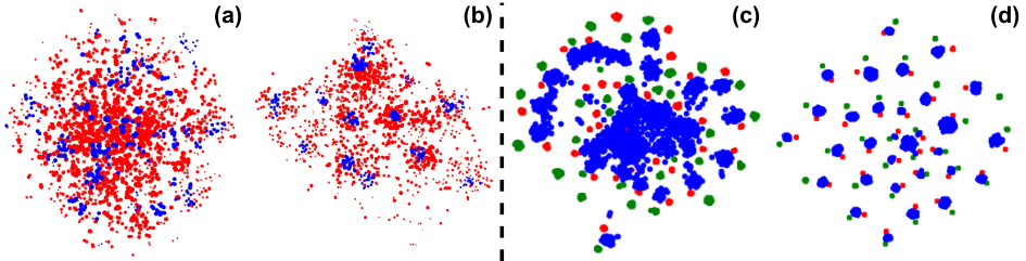
Qualitative Visualization. We use t-SNE [Van der Maaten and Hinton, 2008] to visualize the features produced by source-pretrained models (i.e. No-Adapt) and our models (i.e. Fully-Adapted), and the results are shown in Fig. 5, where the left part is about Single-Source and the right part is about Multi-Source. Fig. 5a and Fig. 5c are results before adaptation, while Fig. 5b and Fig. 5d are results after adaptation. All of these features are produced by Resnet-based source models and target models. From them, we can observe that after adaptation, the data points with varied colors (i.e., from different domains) formmultiple clear clusters and are no longer in chaos, which demonstrates the effectiveness of our proposed method RAIN.

| Single-Source | A→D | Ar→Rw | Syn→Real |
|---|---|---|---|
| w/o Lpm & Lsd & Lwg (baseline) | 90.2 | 79.3 | 76.0 |
| w/ Lpm | 91.6 (↑1.4) | 80.4 (↑1.1) | 77.7 (↑1.7) |
| w/ Lsd | 90.8 (↑0.6) | 79.7 (↑0.4) | 77.0 (↑1.0) |
| w/ Lpm & Lsd | 91.9 (↑1.7) | 81.0 (↑1.7) | 78.9 (↑2.9) |
| w/ Lsd & Lwg | 93.1 (↑2.9) | 81.6 (↑2.3) | 81.7 (↑5.7) |
| RAIN (Lpm + Lsd + Lwg) | 93.8 (↑3.6) | 82.8 (↑3.5) | 82.7 (↑6.7) |
| Multi-Source | →A | →P | →Ar |
| w/o Lpm & Lsd & Lwg (baseline) | 74.9 | 78.6 | 72.1 |
| w/ Lpm | 76.5 (↑1.6) | 80.2 (↑1.6) | 73.3 (↑1.2) |
| w/ Lsd | 75.4 (↑0.5) | 79.4 (↑0.8) | 73.0 (↑0.9) |
| w/ Lpm & Lsd | 77.7 (↑2.8) | 80.8 (↑2.2) | 74.5 (↑2.4) |
| w/ Lsd & Lwg | 78.0 (↑3.1) | 81.2 (↑2.6) | 74.6 (↑2.5) |
| RAIN (Lpm + Lsd + Lwg) | 79.8 (↑4.9) | 82.0 (↑3.4) | 76.0 (↑4.1) |
5 Conclusion
In this paper, we propose a method named RegulArization on Input and Network (RAIN) for Black-Box domain adaptation. We propose a new data augmentation technique called Phase MixUp to regularize the data input, thus encouraging class consistency for better target representations. We also propose Subnetwork Distillation as a network-level regularization technique to transfer knowledge from the target subnetwork to the full target network, hence learning diverse target representations and calibrating the full network. Comprehensive experiments on several datasets testify RAIN's efficacy in both Single-Source and Multi-Source settings, together with detailed quantitative and qualitative analysis.
| Single-Source | A→D | Ar→Cl | Syn→Real |
|---|---|---|---|
| SD-SHOT | 89.2 | 50.1 | 74.5 |
| SD-SHOT w/ MixUp | 89.5 (+0.3) | 50.1 (+0.0) | 73.6 (-0.9) |
| SD-SHOT w/ CutMix | 89.0 (-0.2) | 49.8 (-0.3) | 74.2 (-0.3) |
| SD-SHOT w/ RandAugment | 89.4 (+0.2) | 50.3 (+0.2) | 74.7 (+0.2) |
| SD-SHOT w/ Phase MixUp | 90.8 (+1.6) | 50.7 (+0.6) | 75.2 (+0.7) |
| DINE-full w/o MixUp | 90.9 | 52.9 | 76.3 |
| DINE-full (w/ MixUp by default) | 91.7 (+0.8) | 54.2 (+1.3) | 77.3 (+1.0) |
| DINE-full w/ CutMix | 91.4 (+0.5) | 53.8 (+0.8) | 77.1 (+0.8) |
| DINE-full w/ RandAugment | 92.0 (+1.1) | 54.4 (+1.5) | 77.3 (+1.0) |
| DINE-full w/ Phase MixUp | 92.8 (+1.9) | 55.0 (+2.1) | 77.6 (+1.3) |
| Multi-Source | →A | →P | →Ar |
| SD-DECISION | 66.6 | 74.1 | 62.5 |
| SD-DECISION w/ MixUp | 66.5 (-0.1) | 74.3 (+0.2) | 62.0 (-0.5) |
| SD-DECISION w/ CutMix | 67.2 (+0.6) | 74.7 (+0.6) | 62.2 (-0.3) |
| SD-DECISIONw/ RandAugment | 68.6 (+2.0) | 74.8 (+0.7) | 63.0 (+0.5) |
| SD-DECISIONw/ Phase MixUp | 69.9 (+3.3) | 75.6 (+1.5) | 64.5 (+2.0) |
| DINE-full w/o MixUp | 75.3 | 78.8 | 73.0 |
| DINE-full (w/ MixUp by default) | 77.1 (+1.8) | 79.7 (+0.9) | 74.9 (+1.9) |
| DINE-full w/ CutMix | 75.0 (-0.3) | 77.4 (-1.4) | 73.5 (+0.5) |
| DINE-full w/ RandAugment | 78.1 (+2.8) | 80.6 (+1.8) | 74.5 (+1.5) |
| DINE-full w/ Phase MixUp | 78.8 (+3.5) | 81.3 (+2.5) | 75.6 (+2.6) |
@inproceedings{ijcai2023p458,
  title     = {RAIN: RegulArization on Input and Network for Black-Box Domain Adaptation},
  author    = {Peng, Qucheng and Ding, Zhengming and Lyu, Lingjuan and Sun, Lichao and Chen, Chen},
  booktitle = {Proceedings of the Thirty-Second International Joint Conference on
               Artificial Intelligence, {IJCAI-23}},
  publisher = {International Joint Conferences on Artificial Intelligence Organization},
  editor    = {Edith Elkind},
  pages     = {4118--4126},
  year      = {2023},
  month     = {8},
  note      = {Main Track},
  doi       = {10.24963/ijcai.2023/458},
  url       = {https://doi.org/10.24963/ijcai.2023/458},
}
TY - CPAPER TI - RAIN: RegulArization on Input and Network for Black-Box Domain Adaptation AU - Peng, Qucheng AU - Ding, Zhengming AU - Lyu, Lingjuan AU - Sun, Lichao AU - Chen, Chen T2 - Proceedings of the Thirty-Second International Joint Conference on Artificial Intelligence, IJCAI-23 PB - International Joint Conferences on Artificial Intelligence Organization PY - 2023 SP - 4118 EP - 4126 DO - 10.24963/ijcai.2023/458 UR - https://doi.org/10.24963/ijcai.2023/458 ER -Copied
Machine-readable versions of this paper, for tools and AI agents:





