
Graph-based Semi-supervised Local Clustering with Few Labeled Nodes
Proceedings of the Thirty-Second International Joint Conference on Artificial Intelligence. Main Track. Pages 4190-4198.
https://doi.org/10.24963/ijcai.2023/466
Keywords
- Data Mining: DM: Mining graphs
- Machine Learning: ML: Clustering
- Machine Learning: ML: Semi-supervised learning
Abstract
Local clustering aims at extracting a local structure inside a graph without the necessity of knowing the entire graph structure. As the local structure is usually small in size compared to the entire graph, one can think of it as a compressive sensing problem where the indices of target cluster can be thought as a sparse solution to a linear system. In this paper, we apply this idea based on two pioneering works under the same framework and propose a new semi-supervised local clustering approach using only few labeled nodes. Our approach improves the existing works by making the initial cut to be the entire graph and hence overcomes a major limitation of the existing works, which is the low quality of initial cut. Extensive experimental results on various datasets demonstrate the effectiveness of our approach.
- [Abbe and Sandon, 2015] Emmanuel Abbe and Colin San- don. Recovering communities in the general stochastic block model without knowing the parameters. In Ad- vances in Neural Information Processing Systems, pages 676-684, 2015.
- [Abbe, 2018] Emmanuel Abbe. Community detection and stochastic block models: Recent developments. Journal of Machine Learning, 18(177):1-86, 2018.
- [Adamic and Glance, 2005] Lada A. Adamic and Natalie Glance. The political blogosphere and the 2004 us elec- tion: Divided they blog. In Proceedings of the 3rd Inter- national Workshop on Link Discovery, pages 36-43, 2005.
- [Andersen et al., 2006] Reid Andersen, Fan Chung, and Kevin Lang. Local graph partitioning using pagerank vec- tors. IEEE Symposium on Foundations of Computer Sci- ence, pages 475-486, 2006.
- [Andersen et al., 2007] Reid Andersen, Fan Chung, and Kevin Lang. Using pagerank to locally partition a graph. Internet Mathematics, 4(1):35-64, 2007.
- [Basu et al., 2004] Sugato Basu, Arindam Banerjee, and Raymond J. Mooney. Active semi-supervision for pair- wise constrained clustering. In Proceedings of the SIAM International Conference on Data Mining, pages 333-344, 2004.
- [Blumensath and Davies, 2009] Thomas Blumensath and Mike E. Davies. Iterative hard thresholding for com- pressed sensing. Applied and computational harmonic analysis, 27(3):265-274, 2009.
- [Candès et al., 2006] Emmanuel J. Candès, Justin Romberg, and Terence Tao. Robust uncertainty principles: Exact signal reconstruction from highly incomplete frequency information. IEEE Transactions on information theory, 52(2):489-509, 2006.
- [Candès et al., 2008] Emmanuel J. Candès, Michael B. Wakin, and Stephen P. Boyd. Enhancing sparsity by reweighted ℓ 1 minimization. Journal of Fourier analysis and applications, 14(5):877-905, 2008.
- [Chung, 1997] Fan Chung. Spectral Graph Theory, vol- ume 92. American Mathematical Society, 1997.
- [Dai and Milenkovic, 2009] Wei Dai and Olgica Milenkovic. Subspace pursuit for compressive sensing signal recon- struction. IEEE Transactions on Information Theory, 55(5):2230-2249, 2009.
- [Dhillon et al., 2004] Inderjit S. Dhillon, Yuqiang Guan, and Brian Kulis. Kernel k-means: spectral clustering and nor- malized cuts. In Proceedings of the tenth ACM SIGKDD Conference, pages 551-556, 2004.
- [Ding et al., 2001] Chris HQ. Ding, Xiaofeng He, Hongyuan Zha, Ming Gu, and Horst D. Simon. A min-max cut algo- rithm for graph partitioning and data clustering. In Pro- ceedings of 2001 IEEE International Conference on Data Mining, pages 107-114, 2001.
- [Donoh, 2006] David L. Donoh. Compressed sensing. IEEE Transactions on Information Theory, 52(4):1289-1306, 2006.
- [Ester et al., 1996] Martin Ester, Hans-Peter Kriegel, Jörg Sander, and Xiaowei Xu. A density-based algorithm for discovering clusters in large spatial databases with noise. In kdd, 96(34):226-231, 1996.
- [Feng et al., 2022] Renzhong Feng, Aitong Huang, Ming- Jun Lai, and Zhaiming Shen. Reconstruction of sparse polynomials via quasi-orthogonal matching pur- suit method. Journal of Computational Mathematics, 41(1):18-38, 2022.
- [Fountoulakis et al., 2018] Kimon Fountoulakis, David F. Gleich, and Michael W. Mahoney. A short introduction to local graph clustering methods and software. arXiv preprint arXiv:1810.07324, 2018.
- [Fountoulakis et al., 2019] Kimon Fountoulakis, Farbod Roosta-Khorasani, Julian Shun, and Xiang Cheng. Varia- tional perspective on local graph clustering. Mathematical Programming, 174(1):553-573, 2019.
- [Fountoulakis et al., 2020] Kimon Fountoulakis, Di Wang, and Shenghao Yang. p-norm flow diffusion for local graph clustering. International Conference on Machine Learn- ing, pages 3222-3232, 2020.
- [Grant et al., 2020] Michael Grant, Stephen Boyd, and Yinyu Ye. CVX: Matlab software for disciplined convex programming, version 2.2. available: http://cvxr.com/cvx, 2020. Link
- [Guo et al., 2017] Xifeng Guo, Long Gao, Xinwang Liu, and Jianping Yin. Improved deep embedded clustering with local structure preservation. In Proceedings of the Inter- national Joint Conference on Artificial Intelligence, pages 1573-1759, 2017. IJCAI
- [Huang et al., 2012] Hsin-Chien Huang, Yung-Yu Chuang, and Chu-Song Chen. Affinity aggregation for spectral clustering. IEEE Conference on Computer Vision and Pat- tern Recognition, pages 773-780, 2012.
- [Huang et al., 2015] Jin Huang, Feiping Nie, and Heng Huang. A new simplex sparse learning model to measure data similarity for clustering. In Proceedings of the 24th International Conference on Artificial Intelligence, pages 3569-3575, 2015. IJCAI
- [Hui et al., 2015] Binyuan Hui, Pengfei Zhu, and Qinghua Hu. Collaborative graph convolutional networks: Unsu- pervised learning meets semi-supervised learning. In Pro- ceedings of the AAAI Conference on Artificial Intelligence, volume 34, pages 4215-4222, 2015.
- [Kang et al., 2021] Zhao Kang, Chong Peng, Qiang Cheng, Xinwang Liu, Xi Peng, Zenglin Xu, and Ling Tian. Struc- tured graph learning for clustering and semi-supervised classification. Pattern Recognition, 110, 2021.
- [Kloster and Gleich, 2014] Kyle Kloster and David F. Gle- ich. Heat kernel based community detection. In Proceed- ings of the 20th ACM SIGKDD international Conference on Knowledge Discovery and Data Mining, pages 1386- 1395, 2014.
- [Kulis et al., 2005] Brian Kulis, Sugato Basu, Inderjit Dhillon, and Raymond Mooney. Semi-supervised graph clustering: a kernel approach. In Proceedings of the 22nd International Conference on Machine Learning, pages 457-464, 2005.
- [Lai and Mckenzie, 2020] Ming-Jun Lai and Daniel Mcken- zie. Compressive sensing approach to cut improvement and local clustering. SIAM Journal on Mathematics of Data Science, 2(2):368-395, 2020.
- [Lai and Shen, 2023] Ming-Jun Lai and Zhaiming Shen. A compressed sensing based least squares approach to semi- supervised local cluster extraction. Journal of Scientific Computing, 94(63), 2023.
- [Lai and Wang, 2021] Ming-Jun Lai and Yang Wang. Sparse Solutions of Underdetermined Linear Systems and Their Applications. Society for Industrial and Applied Mathe- matics, 2021.
- [Lang and Rao, 2004] Kevin Lang and Satish Rao. A flow- based method for improving the expansion or conductance of graph cuts. International Conference on Integer Pro- gramming and Combinatorial Optimization, pages 325- 337, 2004.
- [Li, 2016] Haifeng Li. Improved analysis of sp and cosamp under total perturbations. EURASIP Journal on Advances in Signal Processing, 1:1-6, 2016.
- [Liu et al., 2012] Guangcan Liu, Zhouchen Lin, Shuicheng Yan, Ju Sun, Yong Yu, and Yi Ma. Robust recovery of sub- space structures by low-rank representation. IEEE Trans- actions on Pattern Analysis and Machine Intelligence, 35(1):171-184, 2012.
- [Luxburg, 2007] Ulrike Von Luxburg. A tutorial on spec- tral clustering. Statistics and Computing, 17(4):395-416, 2007.
- [MacQueen, 1967] J. MacQueen. Classification and analysis of multivariate observations. In Proceedings of the Fifth Berkeley Symposium on Mathematical Statistics and Prob- ability, pages 281-297, 1967.
- [Mckenzie and Damelin, 2019] Daniel Mckenzie and Steven Damelin. Power weighted shortest paths for clustering eu- clidean data. Foundations of Data Science, 1(3):307-327, 2019.
- [Needell and Tropp, 2009] Deanna Needell and Joel A. Tropp. Cosamp: Iterative signal recovery from incomplete and inaccurate samples. Applied and Computational Har- monic Analysis, 26(3):301-321, 2009.
- [Ng et al., 2001] Andrew Ng, Michael Jordan, and Yair Weiss. On spectral clustering: Analysis and an algorithm. Advances in neural information processing systems, 14, 2001.
- [Nielsen, 2016] Frank Nielsen. Hierarchical clustering. In- troduction to HPC with MPI for Data Science., pages 195- 211, 2016.
- [Orecchia and Zhu, 2014] Lorenzo Orecchia and Zeyuan Allen Zhu. Flow-based algorithms for local graph clustering. In Proceedings of the twenty-fifth annual ACM-SIAM symposium on Discrete algorithms, pages 1267-1286, 2014.
- [Ren et al., 2019] Yazhou Ren, Kangrong Hu, Xinyi Dai, Lili Pan, Steven CH Hoi, and Zenglin Xu. Semi- supervised deep embedded clustering. Neurocomputing, 325:121-130, 2019.
- [Shi et al., 2019] Pan Shi, Kun He, David Bindel, and John E. Hopcroft. Locally-biased spectral approxima- tion for community detection. Knowledge-Based Systems, 164:459-472, 2019.
- [Tibshirani, 1996] Robert Tibshirani. Regression shrinkage and selection via the lasso. Journal of the Royal Statistical Society: Series B (Methodological), 58:267-288, 1996.
- [Tropp, 2004] Joel A. Tropp. Greed is good: Algorithmic results for sparse approximation. IEEE Transactions on Information Theory, 50:2231-2242, 2004.
- [Tsitsulin et al., 2020] Anton Tsitsulin, John Palowitch, Bryan Perozzi, and Emmanuel Müller. Graph clus- tering with graph neural networks. arXiv preprint arXiv:2006.16904, 2020.
- [Veldt et al., 2016] Nate Veldt, David Gleich, , and Michael Mahoney. A simple and strongly-local flow-based method for cut improvement. In Proceedings of the Interna- tional Conference on Machine Learning, pages 1938- 1947, 2016.
- [Veldt et al., 2019] Nate Veldt, Christine Klymko, and David F. Gleich. Flow-based local graph clustering with better seed set inclusion. In Proceedings of SIAM Interna- tional Conference on Data Mining, pages 378-386, 2019.
- [Wang et al., 2017] Di Wang, Kimon Fountoulakis, Monika Henzinger, Michael W. Mahoney, and Satish Rao. Capac- ity releasing diffusion for speed and locality. In Proceed- ings of the International Conference on Machine Learn- ing, pages 3598-3607, 2017.
- [Wilson et al., 2014] James D. Wilson, Simi Wang, Peter J. Mucha, Shankar Bhamidi, and Andrew B. Nobel. A test- ing based extraction algorithm for identifying significant communities in networks. The Annals of Applied Statis- tics, 8:1853-1891, 2014.
- [Xie et al., 2016] Junyuan Xie, Ross Girshick, and Ali Farhadi. Unsupervised deep embedding for clustering analysis. In Proceedings of the International Conference on Machine Learning, pages 478-487, 2016.
- [Zelnik-Manor and Perona, 2004] Lihi Zelnik-Manor and Pietro Perona. Self-tuning spectral clustering. Advances in Neural Information Processing Systems, 17, 2004.
References were extracted automatically from the PDF and may contain errors.
Full text extracted automatically from the PDF; figures, tables and equations may differ. The PDF is the version of record.
1 Introduction
Being able to learn from data by investigating its underlying pattern, and separate data into different groups or clusters based on their latent similarity and differences is one of the main interests in machine learning and artificial intelligence. There are many clustering phenomena across disciplines such as social science, health science, and engineering. Through the past few decades, traditional clustering problem has been studied a lot and many algorithms have been developed, such as k-means clustering [MacQueen, 1967], hierarchical clustering [Nielsen, 2016], and density based clustering [Ester et al., 1996]. For graph structured data or the data which can be converted into a graph structure by applying some techniques (e.g. K-NN auxiliary graph), it is natural to consider the task as a graph clustering problem.
Traditional graph clustering problem assumes the underlying data structure as a graph where data points are the nodes and the connections between data points are the edges. It assigns each node into a unique cluster, assuming there are no multi-class assignments. For nodes with high connection density, they are considered in the same cluster, and for nodes with low connection density, they are considered in different clusters. Since the task is to learn the clustering patterns by investigating the underlying graph structure, it is an unsupervised learning task. Many unsupervised graph clustering algorithms have been developed through decades. For example, spectral clustering [Ng et al., 2001], which is based on the eigen-decomposition of Laplacian matrices of either weighted or unweighted graphs. Based on this, many variants of spectral clustering algorithms have been proposed, such as [Zelnik-Manor and Perona, 2004] and [Huang et al., 2012]. Another category is the graph partition based method such as finding the optimal cut [Dhillon et al., 2004; Ding et al., 2001]. It is worthy noting that spectral clustering and graph partition have the same essence, see [Luxburg, 2007]. Spectral clustering has become one of the popular modern clustering algorithms since it enjoys the advantage of exploring the intrinsic data structures. It is simple to implement, and it often outperforms the traditional algorithm such as k-means. However, one of the main drawbacks of spectral clustering is its high computational cost, so it is usually not applicable to large datasets. Meanwhile, the spectral clustering method does not perform well on the auxiliary graphs which are generated from certain shapes of numerical data, e.g., elongated band shape data and moon shape data. In addition, many other clustering methods have been developed, such as the low rank and sparse representations based methods [Liu et al., 2012; Huang et al., 2015], deep embedding based methods [Xie et al., 2016], and graph neural network based methods [Hui et al., 2015; Tsitsulin et al., 2020]. Besides the unsupervised way, some semi-supervised graph clustering methods have also been proposed [Kulis et al., 2005; Kang et al., 2021; Ren et al., 2019].
These clustering algorithms, whether unsupervised or semi-supervised, are all global clustering algorithms, which means that the algorithms output all the clusters simultaneously. However, it is often to people's interests in only finding a single target cluster which contains the given labels, without worried too much about how the remaining part of graph will be clustered. Such an idea is very useful in detecting small-scale structure in a large-scale graph. This type of problem is referred to as local clustering or local cluster extraction. Most of the current local clustering algorithms aim at finding the best cut from the graph, for example, [Veldt et al., 2019; Fountoulakis et al., 2020; Orecchia and Zhu, 2014]. It is worth pointing out that
[Fountoulakis et al., 2018] have kindly put several methods of local graph clustering into software, including both the spectral methods [Andersen et al., 2006; Fountoulakis et al., 2019] and flow-based methods [Lang and Rao, 2004; Veldt et al., 2016; Wang et al., 2017]. More recently, new approaches for making the cut of graph based on the idea of compressive sensing are proposed in [Lai and Mckenzie, 2020] and [Lai and Shen, 2023], where they took a novel perspective by considering the way of finding the optimal cut as an improvement from an initial cut via finding a sparse solution to a linear system. However, the performances of their approaches will heavily depend on the quality of initial cut.
In this paper, based on the idea of compressive sensing, we propose a semi-supervised local clustering method using only few labeled nodes from the target cluster, with theoretical guarantees. Our approach improves the existing works by making the initial cut to be the entire graph and hence overcomes the issue that missing vertices of the target cluster from the initial cut are not recoverable in the later stage. Extensive experiments are conducted on various benchmark datasets to show our approach outperforms its counterparts [Lai and Mckenzie, 2020; Lai and Shen, 2023]. Results also show that our approach is favorable than many other state-ofthe-art semi-supervised clustering algorithms.
2 Preliminaries
2.1 Graph Notations and Concepts
We adopt the standard notations for graph G = (V, E), where V is the set of all vertices and E is the set of all edges. In the case that the size of graph equals to n, we identify V = {1, 2, · · · , n} = [n]. For a graph G with k non-overlapping underlying clusters C1, C2, · · · , Ck, we use ni to indicate the size of Ci where i = 1, 2, · · · , k. Without loss of generality, let us assume n1 ≤ n2 ≤ · · · ≤ nk. Furthermore, we use matrix A to denote the adjacency matrix of graph G, and use D to denote the diagonal matrix where each diagonal entry in D is the degree of the corresponding vertex. In addition, we define the notion called graph Laplacian.
Definition 1. The unnormalized graph Laplacian of graph G is defined as L = D - A. The symmetric graph Laplacian of graph G is defined as Lsym := I - D-1/2AD-1/2 and the random walk graph Laplacian is defined as Lrw := I - D-1A.
For the scope of our problem, we will only focus on Lrw for the rest of discussion and we will use L to denote Lrw for the concise of notation. Recall the following fundamental result from spectral graph theory. We omit the proof by referring to [Chung, 1997] and [Luxburg, 2007].
Lemma 1. Let G be an undirected graph with non-negative weights. The multiplicity k of the eigenvalue zero of L equals to the number of connected components C1,C2, · · · ,Ck in G, and the indicator vectors 1C1 , · · · , 1Ck ∈ Rn on these components span the kernel of L.
For a graph G with underlying structure which separates vertices into different clusters, we can write G = Gin ∪Gout , where Gin = (V,Ein ) and Gout = (V,Eout ). Here Ein is the set of all intra-connection edges within the same cluster, Eout is the set of all inter-connection edges between different clusters. We use Ain and Aout to denote the adjacency matrices associated with Gin and Gout respectively, and use Lin and Lout to denote the Laplacian matrices associated with Gin and Gout respectively. From their definitions, we can easily see Lin is in a block diagonal form if the vertices are sorted according to their memberships. It is worthwhile to point out that A = Ain + Aout but L ̸= Lin + Lout in general.
| Symbols | |
|---|---|
| G |G| V |V | C1 Γ T E Ein Eout Gin Gout A Ain Aout L Lin Lout LC Lin C |M| ∥M∥2 |v| ∥v∥2 1C △ Ker Span Ls(v) | Interpretations A general graph of interest Size of G Set of vertices of graph G Size of V Target Cluster Set of Seeds Removal set from V Set of edges of graph G Subset of E which consists only intra-connection edges Subset of E which consists only inter-connection edges Subgraph of G on V with edge set Ein Subgraph of G on V with edge set Eout Adjacency matrix of graph G Adjacency matrix of graph Gin Adjacency matrix of graph Gout Random walk graph Laplacian of G Random walk graph Laplacian of Gin Random walk graph Laplacian of Gout submatrix of L with column indices C ⊂ V submatrix of Lin with column indices C ⊂ V Entrywised absolute value operation on matrix M ∥ · ∥2 norm of matrix M Entrywised absolute value operation on vector v ∥ · ∥2 norm of vector v. Indicator vector on subset C ⊂ V Set symmetric difference Kernel of the linear map induced by a matrix Spanning set of a set of vectors {i ∈ [n] : vi among s largest-in-magnitude entries in v} |
Remark 1. We introduce these notations in order for the convenience of our discussion in the later sections. Note that in reality we will have no assurance about which cluster each individual vertex belongs to, so we have no access to Ain and Lin . What we have access to are A and L.
Furthermore, for a set S, we use |S| to denote its size. For a matrix M or vector v, we use |M| or |v| to denote the matrix or vector where each of its entry is replaced by the absolute value. For a matrix M and a set S ⊂ V , we use MS to denote the submatrix of M where the columns of MS consist of only the indices in S. For convenience, we summarize the notations being used throughout this paper in Table 1.
2.2 Compressive Sensing
Recall that ∥·∥0 counts the number of nonzero components in a vector. The idea of compressive sensing comes from solving the optimization problem:
where Φ ∈ Rm×n is called sensing matrix, y ∈ Rn is called measurement vector. The goal is to recover the sparse solution x ∈ Rn under some constraints. It can be reformulated as solving:
Its idea was first introduced by Dohono [Donoh, 2006] and Cand`es, Romberg, Tao [Cand`es et al., 2006]. Since then, many algorithms have been developed to solve (1) or (2), including the greedy based approaches such as orthogonal matching pursuit (OMP) [Tropp, 2004] and its variants, quasi-orthogonal matching pursuit (QOMP) [Feng et al., 2022], thresholding based approaches such as iterative hard thresholding [Blumensath and Davies, 2009], compressive sensing matching pursuit (CoSAMP) [Needell and Tropp, 2009], and subspace pursuit [Dai and Milenkovic, 2009], etc,. Note that (1) is NP-hard because of the appearance of zero norm. Therefore it is sometimes convenient to solve its ℓ1 convex relaxation:
Algorithms such as LASSO [Tibshirani, 1996], CVX [Grant et al., 2020], and reweighted ℓ1-minimization [Cand`es et al., 2008] fall into this category. We do not analyze further here. The monograph [Lai and Wang, 2021] gives a comprehensive summary of these algorithms.
It is worthwhile to mention one of the key concepts in compressive sensing, Restricted Isometry Property (RIP), which guarantees a good recovery of the solution to (1).
Definition 2. Let Φ ∈ Rm×n , 1 ≤ s ≤ n be an integer. Suppose there exists a constant δs ∈ (0, 1) such that
for all x ∈ Rn with ∥x∥0 ≤ s. Then the matrix Φ is said to have the Restricted Isometry Property (RIP). The smallest constant δs which makes (4) hold is called the Restricted Isometry Constant (RIC).
Another very important aspect which makes compressive sensing very useful is its robustness to noise. Suppose we try to solve the linear system y = Φx given the measurement y and sensing matrix Φ. It is possible that we only have access to a noise version of Φ, say ˜Φ = Φ + ϵ1, and also only have access to a noise version of y, say ˜y = y + ϵ2. Therefore, instead of solving y = Φx, what we solve in reality is ˜y = ˜Φ˜x. However, if ϵ1, ϵ2 are both small in some sense, and the sensing matrix Φ satisfies certain conditions, then we will have ˜x ≈ x. There are plenty of ways to solve ˜x given ˜Φ and ˜y, what we will be focusing on is subspace pursuit [Dai and Milenkovic, 2009]. Theorem 2.5 in [Lai and Mckenzie, 2020] and Corollary 1 in [Li, 2016] gives a result about how close ˜x and x can be based on the conditions of ˜Φ, Φ, ˜y, y, which we will apply later in our theoretical analysis part.
2.3 Problem Statement
For convenience, let us assume the target cluster is the first cluster C1 for the rest of discussion. Now let us formally state the local clustering task that we are interested in:
Suppose G = (V,E) is a graph with underlying cluster C1, · · · , Ck where V = ∪ni=1Ci, Ci ∩ Cj = ∅ for 1 ≤ i, j ≤ k, i ̸= j. Given a set of labeled vertices Γ ⊂ C1, which we call them seeds, assuming the size of Γ is small relative to the size of C1. The goal is to extract all the vertices in the target cluster C1.
3 Local Clustering via Compressive Sensing
The local clustering task can be considered as a compressive sensing problem in the following way. Suppose the vertices have been sorted according to their memberships, i.e., the first n1 rows and columns in Lin corresponds to all the vertices in C1, the last nk rows and columns corresponds to all the vertices in Ck, etc,.
Let Lin -1 be the matrix obtained from Lin by deleting the first column fromC1. For this particular graph, all the clusters have size three, the symbol ∗ equals to -1/2, and all the other entries in the off-diagonal blocks equal to zero.
Let yin be the row sum vector of Lin -1 . Then the desired solution to the compressive sensing problem
is x∗ = (1, 1, 0, · · · , 0)′ . The significance of this formulation is that the nonzero components in x∗ correspond to the indices of vertices which belong to the target cluster C1. This gives us the intuitive idea of how to apply compressive sensing for solving local clustering problem.
As noted in Remark 1, we usually do not have access to Lin or Lin -1 , what we do have access to are L and L-1. We can relax the exact equality condition to approximately equal to, so the problem becomes
where y is the row sum vector of L-1. Let x# be the solution to (7). Suppose the graph has a good underlying clusters structure, in other words, the entries in the off-diagonal block of L-1 have very small magnitude, i.e., L-1 ≈ Lin -1 . Then we should have y ≈ yin , and hence the difference between x# and x∗ should be small in certain sense. We can then use some cutoff number R ∈ (0, 1) to separate the coordinates of x# and therefore extract the target cluster from the entire graph.
3.1 Main Algorithm
In general, we can remove more than just one column. That is, we remove a set T ⊂ V in a somewhat smart way, with the hope that T ⊂ C1, and then we solve
Algorithm 1 Compressive Sensing of Local Cluster Extraction (CS-LCE)
Input: Adjacency matrix A, and a small set of seeds Γ ⊂ C1 Parameter: Estimated size ˆn1 ≈ |C1|, random walk threshold parameter ϵ ∈ (0, 1), random walk depth t ∈ Z+, sparsity parameter γ ∈ [0.1, 0.5], rejection parameter R ∈ [0.1, 0.9]
Output: The target cluster C1
- 1: Compute P = AD-1 , v0 = D1Γ, and L = I -D-1A.
- 2: Compute v(t) = P tv(0) .
- 3: Define Ω = L(1+ϵ)ˆn1 (v(t) ).
- 4: Let T be the set of column indices of γ · |Ω| smallest components of the vector |L⊤Ω | · |L1Ω|.
- 5: Set y := L1V \T . Let x# be the solution to
obtained by using O(logn) iterations of Subspace Pursuit [Dai and Milenkovic, 2009].
- 6: Let W # = {i : x#i > R} .
- 7: return C # 1 =W # ∪ T.
Or equivalently, we solve
where vector y is the row sum vector of LV \T and s is the sparsity constraint.
Naively, if the size of Γ is not too small, then we can just choose T = Γ. However, for the scope of our problem, the size of Γ is assumed to be small relative to the size of C1, therefore this choice does not work well in practice. Instead, we select T based on a heuristic criterion (as described in step 4) on a candidate set Ω which is obtained from a random walk originates from Γ. We also find that the size of T does not matter too much based on our exploration in the experiments. The idea is summarized in Algorithm 1 as CS-LCE. We give a more detailed explanation about several aspects of the algorithm in Remark 2 and Remark 3. More generally, we can apply CS-LCE iteratively to extract all the clusters one at a time.
We would like to point out the major differences between CS-LCE with its counterparts CP+RWT in [Lai and Mckenzie, 2020] and LSC in [Lai and Shen, 2023]. The key difference is that the latter two methods only be able to extract target cluster from the initial cut Ω, since it is assumed that C1 ⊂ Ω in these two methods before extracting all the vertices in C1, and once Ω fails to contain any vertex in C1, there is no chance for CP+RWT or LSC to recover those vertices in the later stage. However, such an assumption is not needed in CS-LCE. Since the sensing matrix in CS-LCE is associated with all the vertices corresponding to V \ T , it is very probable for CS-LCE to still be able to find the vertices which are in C1 but not in Ω.
Remark 2. The purpose of Ω is solely for obtaining the set T , and the vector y is computed by adding up all the columns with indices in the set V \T . This is another key difference between CS-LCE and CP+RWT [Lai and Mckenzie, 2020] and LSC [Lai and Shen, 2023], whereas the latter two methods directly use Ω to obtain y.
Remark 3. The rationale for choosing an iterative approach such as Subspace Pursuit over other sophisticated optimization algorithms for solving (10) comes from the nature of our task. Since the task is clustering, all we need is a relative good estimated solution instead of the exact solution, then we can use a cutoff number R in Algorithm 1 to separate the aimed cluster from the remaining of the graph. Due to the nature of an iterative approach, the convergence is usually fast at the beginning and slow in the end, so we can stop early in the iteration to save the computational cost once the estimated solution is roughly "close enough" to the true solution.
3.2 Theoretical Analysis
For convenience, let us fix γ = 0.4 for the rest of discussion. We want to make sure the output C # 1 from Algorithm 1 is as close to the true cluster C1 as possible. In order to investigate more towards this aspect, let us use x∗ to denote the solution to the unperturbed problem:
where yin = Lin1V \T . Let x# be the solution to (10), the perturbed problem, with γ = 0.4.
Let us first establish the correctness of having x∗ equals to an indicator vector as the solution to (11), and then conclude that x# ≈ x∗ if L ≈ Lin in a certain sense. Once this is established, we will be able to conclude C # 1 ≈ C1. These results are summarized in the following as a series of theorems and lemma.
Theorem 1. Suppose T ⊂ C1. Then x∗ = 1C1\T ∈ R|V |-|T| is the unique solution to (11).
Proof. Note that for yin = Lin1V \T , we can rewrite it as yin = Lin V \T 1 where 1 ∈ R|V |-|T| . It is straightforward to check x∗ = 1C1\T is a solution to (11). The rest is to show it is unique.
Suppose otherwise, then since Lin V \T 1C1\T = yin , we want to find x ∈ R|V |-|T| and x ̸= 1C1\T such that Lin V \T (x - 1) = 0. Without loss of generality, let us assume the columns of L are permuted such that it is in the block diagonal form, i.e.,
Let us now show that Lin C1\T is of full column rank, i.e., the columns of Lin C1\T is linearly independent. We first observe the following fact. By Lemma 1, each of Lin Ci has λ = 0 as an eigenvalue with multiplicity one, and the corresponding eigenspace is spanned by 1Ci . Now suppose by contradiction that the columns of Lin C1\T are linearly dependent, so there exists v ̸= 0 such that Lin C1\T v = 0, or Lin C1\T v + Lin T · 0 = 0. This means that u = (v, 0) is an eigenvector associated to eigenvalue zero, which contradicts the fact that the eigenspace is spanned by 1Ci . Therefore Lin C1\T is of full column rank.
Since Lin C1\T is of full column rank, and Ker(Lin Ci ) = Span{1Ci } for i ≥ 2. We conclude that x - 1 ∈ Ker(Lin V \T ) = Span{1C2 , · · · , 1Cn }. Therefore in order to satisfy ∥x∥0 ≤ 0.6n1, it is easy to see x = 1 - 1C2 - 1C3 - · · · - 1Ck = 1C1\T , which results in a contradiction by our assumption.
The next theorem shows that x∗ and x# are close to each other if L and Lin are close.
Proof. Recall that x# is the output to (10) after O(logn) iterations of Subspace Pursuit. By our assumption on M, we have
Then applying Theorem 2.5 in [Lai and Mckenzie, 2020], we get the desired result.
Lemma 2. Consider K ⊂ [n], any v ∈ Rn , and W # = {i : vi > R}. If ∥1K - v∥2 ≤ D, then |K△W #| ≤ D2 min{(1-R)2 ,R2 } .
Proof. Let U # = [n] \ W #, we can write v = vU # + vW # where vU # and vW # are the components of v supported on U # and W # respectively. Then we have
Therefore ∥1K - v∥2 ≤ D implies |K△W #| ≤ min{(1-R)2 ,R2 } as desired.
Theorem 3. Suppose T ⊂ C1. Then
Proof. It is equivalent to show |C1△C # 1 | ≤ o(n1). Note that x∗ = 1C1\T . By Theorem 2, we get ∥1C1\T - x#∥2 ≤ o(∥1C1\T ∥2) = o(√n1). We then apply Lemma 2 with K = C1 \ T , W # = C # 1 , and v = x# to get |(C1 \ T)△C # 1 | ≤ o(n1). Therefore |C1△C # 1 | ≤ o(n1).
4 Experiments
In this section, we evaluate Algorithm 1 on various synthetic and real datasets and compare its performance with several baselines. For all experiments, we perform 100 individual runs. Additional details about the experiments are provided in the supplement. We make the supplement and code available at: https://github.com/zzzzms/LocalClustering.
Datasets. We use simulated stochastic block model, simulated geometric data with three particular shapes, network data on political blogs[Adamic and Glance, 2005], OptDigits 1 , AT&T Database of Faces 2 , MNIST 3 , and USPS 4 as our benchmark datasets.
Baselines and Settings. We adopt the LSC [Lai and Shen, 2023], CP+RWT [Lai and Mckenzie, 2020], HKGrow [Kloster and Gleich, 2014], PPR [Andersen et al., 2007], ESSC [Wilson et al., 2014], LBSA [Shi et al., 2019], and several other modern semi-supervised clustering algorithms as our baseline methods. For our experiments of stochastic block model, the only target cluster is the most dominant cluster, i.e., the cluster with the highest connection probability. For all other experiments, all of the clusters are considered as our target clusters, and we apply CS-LCE iteratively to extract all of them. We use Jaccard index to measure the performance of one cluster tasks and use mean accuracy across all clusters to measure the performance of multiple clusters tasks.
1 https://archive.ics.uci.edu/ml/datasets/optical+recognition+of+ handwritten+digits
2 https://git-disl.github.io/GTDLBench/datasets/att face dataset/
3 http://yann.lecun.com/exdb/mnist/
4 https://git-disl.github.io/GTDLBench/datasets/usps dataset/
4.1 Simulated Data
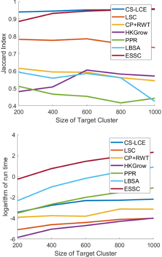
Symmetric Stochastic BlockModel. The stochastic block model is a generative model for random graphs with certain edge densities within and between underlying clusters. The edges within clusters are denser than the edges between clusters. In the case of each cluster has the same size and the intra- and inter-connection probability are the same among all vertices, we have the symmetric stochastic block model SSBM(n, k, p, q). The parameter n is the size of the graph, k is the number of clusters, p is the probability of intraconnectivity, and q is the probability of inter-connectivity. In our experiments, we fix k = 3 and vary n among 600, 1200, 1800, 2400, 3000. We choose p = 5 log n/n, q = logn/n. With five labeled vertices as seeds, we achieve the performances shown in Figure 1. We can see CS-LCE outperforms all other baselines with a reasonable running time.
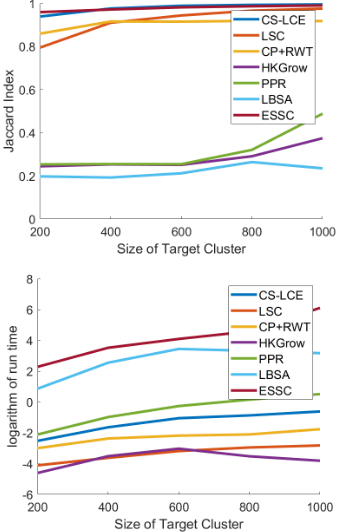
Non-symmetric Stochastic Block Model. In a more general stochastic block model SBM(n, k, P), where n and k are the same as symmetric case. The matrix P indicates the connection probability within each individual cluster and between different clusters. It is worthwhile to note that the information theoretical bound for exact cluster recovery in SBM are given in [Abbe, 2018] and [Abbe and Sandon, 2015]. In our experiments, we fix k = 3, and the size of clusters are chosen as n = (n1, 2n1, 5n1) where n1 is chosen from {200, 400, 600, 800, 1000}. We set the connection probability matrix P = [p, q, q; q, p, q; q, q, p] where p = log2 (8n1)/(8n1) and q = 5 log(8n1)/(8n1). With five labeled vertices as seeds, the clustering performances are shown in Figure 2.
| Datasets | 3 Lines | 3 Circles | 3 Moons |
| LSC | 89.0 (5.53) | 96.2 (3.71) | 85.3 (1.88) |
| CP+RWT | 82.1 (9.06) | 96.1 (5.09) | 85.4 (1.33) |
| CS-LCE | 92.4 (8.13) | 97.6 (4.69) | 96.8 (0.89) |
| Label Ratios | 10 % | 20 % | 30 % |
|---|---|---|---|
| LSC | 94.8 (3.32) | 97.8 (1.18) | 98.2 (0.77) |
| CP+RWT | 93.7 (3.34) | 97.8 (1.44) | 98.3 (0.43) |
| SC | 95.8 (0.00) | 95.8 (0.00) | 95.8 (0.00) |
| CS-LCE | 98.0 (1.90) | 99.1 (0.79) | 99.3 (0.59) |
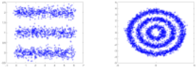
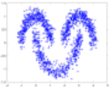
Geometric Data. We also simulated three high dimensional datasets in Euclidean space where the projections of the clusters onto two dimensional plane look like three lines, three circles, or three moons. See Figure 3 for an illustration of them. These datasets are often used as benchmark for data clustering and they are also described in [Mckenzie and Damelin, 2019] with slightly different parameters. Because of the shape of underlying clusters, traditional k-means clustering or spectral clustering fail on these contrived datasets. In our experiments, for each dataset, we randomly select 10 seeds for each of the cluster. The mean accuracy and standard deviation of CS-LCE compared with LSC [Lai and Shen, 2023] and CP+RWT [Lai and Mckenzie, 2020] are given in Table 2. A more detailed description of this simulated dataset is given in the supplement.
4.2 Human Face Images
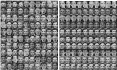
The AT&T Database of Faces contains gray-scale images for 40 different people of pixel size 92 × 112. Images of each person are taken under 10 different conditions, by varying the three perspectives of faces, lighting conditions, and facial expressions. We use part of this dataset by randomly selecting 10 people such that each individual is associated with 10 pictures of themselves. The selected dataset and desired recovery are shown in Figure 4.
The mean accuracy and standard deviation of CS-LCE compared with LSC [Lai and Shen, 2023], CP+RWT [Lai and Mckenzie, 2020], and spectral clustering (SC) are summarized in Table 3. Note that spectral clustering method is unsupervised, hence its accuracy does not affected by the label ratios.
4.3 Network Data
"The political blogosphere and the 2004 US Election" [Adamic and Glance, 2005] dataset contains a list of political blogs that were classified as liberal or conservative with links between blogs. An illustration of this dataset is attached in the supplement. The state-of-the-art result on this dataset is given in [Abbe and Sandon, 2015]. Their simplified algorithm gave a successful classification 37 times out of 40 trials, and each of the successful trials correctly classified all but 56 to 67 of the 1,222 vertices in the graph main component.
In our experiments, given one labeled seed, CS-LCE succeeds 35 trials out of a total of 40 trials. Among these 35 successful trials, the average number of misclassified node in the graph main component is 49, which is comparable to the state-of-the-art result. We note that LSC [Lai and Shen, 2023] also succeeds 35 out of 40 trials, but the average number of misclassified node equals to 55. We also note that CP+RWT [Lai and Mckenzie, 2020] fails on this dataset.
4.4 Digits Data
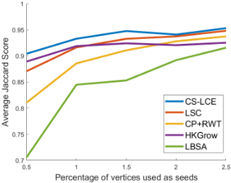
OptDigits. This dataset contains grayscale images of handwritten digits from 0 to 9 of size 8 × 8. There are a total of 5, 620 images and each cluster has approximately 560 images. The average Jaccard index of CS-LCE compared with several other algorithms are shown in Figure 5. we exclude PPR and ESSC in the comparison as they either too slow to run or the accuracy is too low.
MNISTandUSPS. TheMNIST dataset consists of 70, 000 grayscale images of the handwritten digits 0-9 of size 28×28
| Label Ratios | 0.05 % | 0.10 % | 0.15 % |
|---|---|---|---|
| LSC | 77.0 (3.47) | 83.6 (2.76) | 88.8 (2.52) |
| CP+RWT | 74.1 (3.13) | 79.7 (2.43) | 85.0 (2.37) |
| CS-LCE | 85.3 (2.67) | 89.8 (1.91) | 93.2 (1.76) |
| Label Ratios | 0.2 % | 0.3% | 0.4% |
|---|---|---|---|
| LSC | 72.3 (3.54) | 77.1 (3.42) | 80.4 (3.20) |
| CP+RWT | 68.9 (3.17) | 73.3 (2.76) | 76.6 (2.59) |
| CS-LCE | 76.8 (3.37) | 80.1 (3.14) | 84.1 (2.53) |
| MNIST | USPS | |
|---|---|---|
| KM-cst [Basu et al., 2004] | 54.27 | 68.18 |
| AE+KM [MacQueen, 1967] | 74.09 | 70.28 |
| AE+KM-cst [Basu et al., 2004] | 75.98 | 71.87 |
| DEC [Xie et al., 2016] | 84.94 | 75.81 |
| IDEC [Guo et al., 2017] | 83.85 | 75.86 |
| SDEC [Ren et al., 2019] | 86.11 | 76.39 |
| CS-LCE (Ours) | 96.02 | 82.10 |
with approximately 7, 000 images of each digit. The USPS data set contains 9298 grayscale images, obtained from the scanning of handwritten digits from envelopes by the U.S. postal service. We test CS-LCE, LCS, CP+RWT, and several other modern semi-supervised methods on these two datasets, the results are show in Table 4, Table 5 and Table 6. It is worth pointing out that in Table 4 and Table 5, we have only very few labeled data for our tasks. If one uses a neural network method to train for classification of images, then it usually needs more labeled data for training. In Table 6, we compare CS-LCE with several other constraint clustering algorithms. In each constrained clustering algorithms, the total number of pairwise constraints are set to equal to the total data points. Therefore in order to have a fair comparison, we choose a certain amount of labeled data in CS-LCE such that the total pairwise constraints are the same.
5 Conclusions
In this work, we proposed a semi-supervised local clustering approach based on compressive sensing. Our approach improves the disadvantages in prior work under the same framework, and it is shown to be asymptotically correct under certain assumptions of graph structure. Extensive Experiments on various datasets have validated its effectiveness. We hope this work will draw people's interests and bring attentions to this new perspective of local clustering. Potential research directions in the future could be done on developing a more calibrated way of choosing the removal set and investigating how to incorporate compressive sensing into some modern architectures such as deep neural networks.
Acknowledgements
The second author is supported by the Simon Foundation Collaboration Grant #864439. The third author is supported by the U.S. Army Research Office Award under Grant Number W911NF-21-1-0109. We want to thank all the reviewers for their valuable feedback to improve the quality of this paper.
@inproceedings{ijcai2023p466,
  title     = {Graph-based Semi-supervised Local Clustering with Few Labeled Nodes},
  author    = {Shen, Zhaiming and Lai, Ming-Jun and Li, Sheng},
  booktitle = {Proceedings of the Thirty-Second International Joint Conference on
               Artificial Intelligence, {IJCAI-23}},
  publisher = {International Joint Conferences on Artificial Intelligence Organization},
  editor    = {Edith Elkind},
  pages     = {4190--4198},
  year      = {2023},
  month     = {8},
  note      = {Main Track},
  doi       = {10.24963/ijcai.2023/466},
  url       = {https://doi.org/10.24963/ijcai.2023/466},
}
TY - CPAPER TI - Graph-based Semi-supervised Local Clustering with Few Labeled Nodes AU - Shen, Zhaiming AU - Lai, Ming-Jun AU - Li, Sheng T2 - Proceedings of the Thirty-Second International Joint Conference on Artificial Intelligence, IJCAI-23 PB - International Joint Conferences on Artificial Intelligence Organization PY - 2023 SP - 4190 EP - 4198 DO - 10.24963/ijcai.2023/466 UR - https://doi.org/10.24963/ijcai.2023/466 ER -Copied
Machine-readable versions of this paper, for tools and AI agents:





