
Spike Count Maximization for Neuromorphic Vision Recognition
Proceedings of the Thirty-Second International Joint Conference on Artificial Intelligence. Main Track. Pages 4253-4261.
https://doi.org/10.24963/ijcai.2023/473
Keywords
- Computer Vision: CV: Machine learning for vision
- Machine Learning: ML: Classification
Abstract
Spiking Neural Networks (SNNs) are the promising models of neuromorphic vision recognition. The mean square error (MSE) and cross-entropy (CE) losses are widely applied to supervise the training of SNNs on neuromorphic datasets. However, the relevance between the output spike counts and predictions is not well modeled by the existing loss functions. This paper proposes a Spike Count Maximization (SCM) training approach for the SNN-based neuromorphic vision recognition model based on optimizing the output spike counts. The SCM is achieved by structural risk minimization (SRM) and a specially designed spike counting loss. The spike counting loss counts the output spikes of the SNN by using the L0-norm, and the SRM maximizes the distance between the margin boundaries of the classifier to ensure the generalization of the model. The SCM is non-smooth and non-differentiable, and we design a two-stage algorithm with fast convergence to solve the problem. Experiment results demonstrate that the SCM performs satisfactorily in most cases. Using the output spikes for prediction, the accuracies of SCM are 2.12%~16.50% higher than the popular training losses on the CIFAR10-DVS dataset. The code is available at https://github.com/TJXTT/SCM-SNN.
- [Amir et al., 2017] Arnon Amir, Brian Taba, David Berg, Timothy Melano, Jeffrey McKinstry, Carmelo Di Nolfo, Tapan Nayak, Alexander Andreopoulos, Guillaume Gar- reau, Marcela Mendoza, et al. A low power, fully event- based gesture recognition system. In CVPR, 2017.
- [Baldwin et al., 2022] Raymond Baldwin, Ruixu Liu, Mo- hammed Mutlaq Almatrafi, Vijayan K Asari, and Keigo Hirakawa. Time-ordered recent event (tore) volumes for event cameras. IEEE Transactions on Pattern Analysis and Machine Intelligence, pages 1-1, 2022.
- [Bi et al., 2019] Yin Bi, Aaron Chadha, Alhabib Abbas, Ei- rina Bourtsoulatze, and Yiannis Andreopoulos. Graph- based object classification for neuromorphic vision sens- ing. In ICCV, 2019.
- [Bu et al., 2021] Tong Bu, Wei Fang, Jianhao Ding, PengLin Dai, Zhaofei Yu, and Tiejun Huang. Optimal ann-snn conversion for high-accuracy and ultra-low-latency spik- ing neural networks. In ICLR, 2021.
- [Chen et al., 2021] Yanqi Chen, Zhaofei Yu, Wei Fang, Tiejun Huang, and Yonghong Tian. Pruning of deep spik- ing neural networks through gradient rewiring. In IJCAI, 2021. IJCAI
- [Deng and Gu, 2021] Shikuang Deng and Shi Gu. Optimal conversion of conventional artificial neural networks to spiking neural networks. In ICLR, 2021.
- [Deng et al., 2021] Yongjian Deng, Hao Chen, and Youfu Li. Mvf-net: A multi-view fusion network for event-based ob- ject classification. IEEE Transactions on Circuits and Sys- tems for Video Technology, pages 1-1, 2021.
- [Deng et al., 2022a] Shikuang Deng, Yuhang Li, Shanghang Zhang, and Shi Gu. Temporal efficient training of spiking neural network via gradient re-weighting. In ICLR, 2022.
- [Deng et al., 2022b] Yongjian Deng, Hao Chen, Hai Liu, and Youfu Li. A voxel graph cnn for object classification with event cameras. In CVPR, 2022.
- [Ding et al., 2021] Jianhao Ding, Zhaofei Yu, Yonghong Tian, and Tiejun Huang. Optimal ANN-SNN conversion for fast and accurate inference in deep spiking neural net- works. In IJCAI, 2021. IJCAI
- [Fang et al., 2020] Wei Fang, Yanqi Chen, Jianhao Ding, Ding Chen, Zhaofei Yu, Huihui Zhou, Yonghong Tian, and other contributors. Spikingjelly. https://github.com/ fangwei123456/spikingjelly, 2020. Accessed: 2021-11- 21. Link
- [Fang et al., 2021a] Wei Fang, Zhaofei Yu, Yanqi Chen, Tiejun Huang, Timothée Masquelier, and Yonghong Tian. Deep residual learning in spiking neural networks. In NeurIPS, 2021.
- [Fang et al., 2021b] Wei Fang, Zhaofei Yu, Yanqi Chen, Timothée Masquelier, Tiejun Huang, and Yonghong Tian. Incorporating learnable membrane time constant to en- hance learning of spiking neural networks. In ICCV, 2021.
- [Feng et al., 2022] Lang Feng, Qianhui Liu, Huajin Tang, De Ma, and Gang Pan. Multi-level firing with spiking ds- resnet: Enabling better and deeper directly-trained spiking neural networks. In IJCAI, 2022.
- [Kaiser et al., 2020] Jacques Kaiser, Hesham Mostafa, and Emre Neftci. Synaptic plasticity dynamics for deep contin- uous local learning (decolle). Frontiers in Neuroscience, 14:424, 2020.
- [Lee et al., 2020] Chankyu Lee, Syed Shakib Sarwar, Priyadarshini Panda, Gopalakrishnan Srinivasan, and Kaushik Roy. Enabling spike-based backpropagation for training deep neural network architectures. Frontiers in Neuroscience, 14:119, 2020.
- [Li et al., 2017] Hongmin Li, Hanchao Liu, Xiangyang Ji, Guoqi Li, and Luping Shi. Cifar10-dvs: an event-stream dataset for object classification. Frontiers in neuroscience, 11:309, 2017.
- [Li et al., 2021] Yuhang Li, Yufei Guo, Shanghang Zhang, Shikuang Deng, Yongqing Hai, and Shi Gu. Differen- tiable spike: Rethinking gradient-descent for training spik- ing neural networks. In NeurIPS, 2021.
- [Meng et al., 2022] Qingyan Meng, Mingqing Xiao, Shen Yan, Yisen Wang, Zhouchen Lin, and Zhi-Quan Luo. Training high-performance low-latency spiking neural net- works by differentiation on spike representation. In CVPR, 2022.
- [Pei et al., 2019] Jing Pei, Lei Deng, Sen Song, Mingguo Zhao, Youhui Zhang, Shuang Wu, Guanrui Wang, Zhe Zou, Zhenzhi Wu, Wei He, et al. Towards artificial general intelligence with hybrid tianjic chip architecture. Nature, 572(7767):106-111, 2019.
- [Rahiminejad et al., 2022] Ehsan Rahiminejad, Fatemeh Azad, Adel Parvizi-Fard, Mahmood Amiri, and Bernabé Linares-Barranco. A neuromorphic cmos circuit with self-repairing capability. IEEE Transactions on Neural Networks and Learning Systems, 33(5):2246-2258, 2022.
- [Shrestha and Orchard, 2018] Sumit B Shrestha and Garrick Orchard. Slayer: Spike layer error reassignment in time. NeurIPS, 2018.
- [Shrestha et al., 2022] Sumit Bam Shrestha, Longwei Zhu, and Pengfei Sun. Spikemax: Spike-based loss methods for classification. In IJCNN, 2022.
- [Tang et al., 2018] Jianxiong Tang, Na Zhang, and Qia Li. Robust binary classification via ℓ 0 -svm. In ICDM Work- shops, 2018.
- [Tavanaei et al., 2019] Amirhossein Tavanaei, Masoud Gho- drati, Saeed Reza Kheradpisheh, Timothée Masquelier, and Anthony Maida. Deep learning in spiking neural net- works. Neural Networks, 111:47-63, 2019.
- [Tseng, 2001] Paul Tseng. Convergence of a block co- ordinate descent method for nondifferentiable minimiza- tion. Journal of optimization theory and applications, 109(3):475, 2001.
- [Vapnik, 2000] Vladimir Naumovich Vapnik. The Nature of Statistical Learning Theory, Second Edition. Springer, 2000.
- [Wang et al., 2022] Huajun Wang, Yuan-Hai Shao, Sheng- long Zhou, Ce Zhang, and Naihua Xiu. Support vector machine classifier via l 0/1 soft-margin loss. IEEE Trans- actions on Pattern Analysis and Machine Intelligence, 44(10):7253-7265, 2022.
- [Wu et al., 2018] Yujie Wu, Lei Deng, Guoqi Li, Jun Zhu, and Luping Shi. Spatio-temporal backpropagation for training high-performance spiking neural networks. Fron- tiers in neuroscience, 12:331, 2018.
- [Wu et al., 2019a] Jibin Wu, Yansong Chua, Malu Zhang, Qu Yang, Guoqi Li, and Haizhou Li. Deep spiking neural network with spike count based learning rule. In IJCNN, 2019.
- [Wu et al., 2019b] Yujie Wu, Lei Deng, Guoqi Li, Jun Zhu, Yuan Xie, and Luping Shi. Direct training for spiking neu- ral networks: Faster, larger, better. In AAAI, 2019.
- [Wu et al., 2021] Zhenzhi Wu, Hehui Zhang, Yihan Lin, Guoqi Li, Meng Wang, and Ye Tang. Liaf-net: Leaky integrate and analog fire network for lightweight and effi- cient spatiotemporal information processing. IEEE Trans- actions on Neural Networks and Learning Systems, pages 1-14, 2021.
- [Zhang et al., 2022] Duzhen Zhang, Shuncheng Jia, and Qingyu Wang. Recent advances and new frontiers in spik- ing neural networks. In IJCAI, 2022. IJCAI
- [Zheng et al., 2021] Hanle Zheng, Yujie Wu, Lei Deng, Yi- fan Hu, and Guoqi Li. Going deeper with directly-trained larger spiking neural networks. In AAAI, 2021.
References were extracted automatically from the PDF and may contain errors.
Full text extracted automatically from the PDF; figures, tables and equations may differ. The PDF is the version of record.
1 Introduction
Spiking Neural Networks (SNNs) [Tavanaei et al., 2019; Zhang et al., 2022] are bio-inspired models, and neuromorphic data [Amir et al., 2017; Li et al., 2017] is widely used for low-power vision sensing. Since the SNN transmits the information by the spike sequences, the feature maps of SNNs are binary. This advantage makes the SNN-based neuromorphic sensing techniques energy efficient on neuromorphic chips [Pei et al., 2019; Rahiminejad et al., 2022]. However, because the spiking features of SNNs are non-differentiable almost everywhere, the training of SNNs is more difficult than the Artificial Neural Networks (ANNs).
∗Corresponding Author
Two kinds of learning algorithms are widely used to train SNN: a) ANN-to-SNN (ANN2SNN) conversion; b) Spikebased BP training. The ANN2SNN [Bu et al., 2021; Ding et al., 2021; Deng and Gu, 2021] converts a well-trained ANN to its SNN version. Such a technique provides an efficient way to obtain a SNN from a well-trained ANN. However, the spatial-temporal context of the neuromorphic events is not well modeled by the converted SNN, making ANN2SNN mainly focus on the tasks of static images.
To improve the performance of the SNN-based neuromorphic vision tasks, the spike-based BP algorithms [Wu et al., 2018; Wu et al., 2019b; Lee et al., 2020; Deng et al., 2022a] that use the back-propagation (BP) are designed to direct train the SNNs. The surrogate gradient of the spike-based BP enables the gradient calculations of spikes w.r.t the membrane potential so that the BP algorithms can directly be applied for SNN training. Since the spike-based BP training captures the spatial-temporal dynamics of SNNs, the SNN can learn the context of the neuromorphic events. Many efficient BP-based algorithms are proposed to train the SNNs for better performance [Zheng et al., 2021; Li et al., 2021; Fang et al., 2021a; Deng et al., 2022a; Feng et al., 2022]. However, many of them use the mean square error (MSE) or cross-entropy (CE) loss on the membrane potentials of the logit layer to minimize the gap between the spatial-temporal outputs of SNN and the target spike sequences/ground truth labels. The relevance between spike counts and the correct predictions is not well described since optimizing the logit outputs does not always result in more output spike counts [Shrestha et al., 2022]. Although the spiking neurons can be applied to the output of the SNN to generate the spikes for recognition, the training error is updated based on the surrogate gradient. That is, the training process is to minimize the error between the target and differentiable surrogate, which smoothes the discreteness of the spiking output.
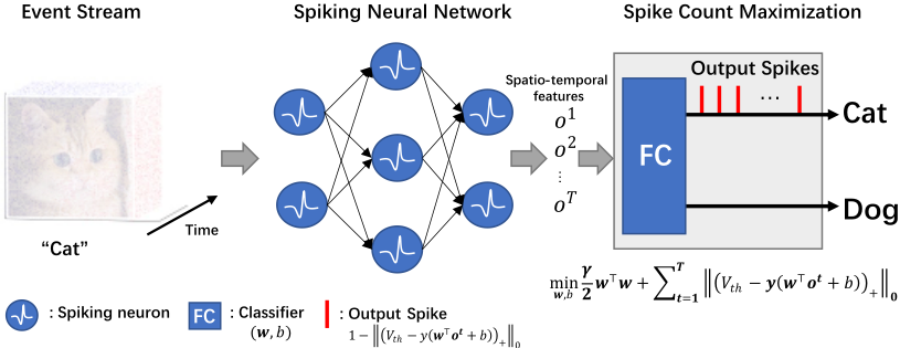
In this paper, we connect the output spike activities with the classification of SNNs. We assume that the output of SNN should activate as many spikes as possible for a correct prediction. Otherwise, the output neurons should be kept at rest. This assumption satisfies the spike counting strategy [Shrestha and Orchard, 2018]. On this basis, we address the SNN training problem by maximizing the number of output spikes for the correct predictions. Specifically, we design a spike counting loss to map each time step's decision output to a binary spike and achieve the training based on structural risk minimization (SRM). The spike counting loss maximizes the number of spikes through time, and the SRM guarantees that each output spike is activated with sufficient confidence.
Our contributions can be summarized as follow:
- We propose the spike counting loss to handle the output spikes of the SNN.
- We propose the spike count maximization (SCM) approach for neuromorphic vision recognition based on the spike counting loss and structural risk minimization.
- We provide iterative solutions to the SCM and then design a two-stage SNN training algorithm.
Experiment results on the popular neuromorphic vision datasets demonstrate that the performance of the SCM is competitive with the popular training loss.
2 Background &RelatedWorks
2.1 Neuromorphic Vision Recognition
The neuromorphic vision datasets are the event streams captured by the bio-inspired vision sensors. The Dynamic Vision Sensor (DVS) [Amir et al., 2017; Li et al., 2017; Bi et al., 2019] is the most popular neuromorphic sensor. It mimics the biological retina and generates a sparse event when a pixel value changes magnitude by a pre-setting threshold. The sparse event stream reduces the cost of energy and bandwidth for real-time transmission. In addition, the event stream's high temporal resolution and dynamic range can provide abundant features for pattern recognition tasks. However, the discontinuous and sparse events make neuromorphic datasets much different from the CMOSbased sensing images. Many ANN-based techniques are designed for neuromorphic vision recognition [Bi et al., 2019; Wu et al., 2021; Deng et al., 2021; Deng et al., 2022b; Baldwin et al., 2022]. However, these methods' good performance relies on the many floating point operations and realvalue features, degenerating the energy efficiency on edge devices or neuromorphic chips.
2.2 Spiking Neural Networks
As shown in Fig. 1, the SNNs encode the input data to the spatial-temporal features. The spiking neuron is the basic component of SNN, and the Leaky Integrate-and-Fire (LIF) neuron is popular for SNN modeling. Given an input sequence {ot }Tt=1 , the dynamic of the LIF neuron is
where τ ∈ (0, 1) is a decay factor, ot denotes the spike and ut is the membrane potential (MP) at t. w is the weight, and b is the bias. The MP integrates the pre-synaptic inputs in a time direction, and the post-synaptic spikes are generated when the MP crosses Vth. After that, the MP is reset to 0. Different from a ReLU-based ANN, the SNN has additional temporal dynamics. In each time step, the activation values are binary rather than a real value of the ReLU activation. The temporal dynamics of SNN enable the processes of the event stream, and the feature maps of every step are binaries. Therefore, the SNNs have more computation-efficient than the ANN for real-time neuromorphic vision recognition.
2.3 Loss Function for SNN Training MP-based Loss
Supposing W ∈ Rd×C and b ∈ RC are the weights and biases of the classifier of the SNN, the Cross-Entropy (CE) and Mean Square Error (MSE) losses for the training of SNN are :
where wj ∈ W, bj ∈ b denote the class center and bias of j, Iyi is a C dimensions one-hot vector of yi, and ¯oi = 1 T T∑ t=1 oti is the average value of the feature over time. Then, the weight of the SNN can be updated by utilizing the spike-based gradient techniques [Wu et al., 2018; Wu et al., 2019b]. The CE and MSE losses collect all decision outputs for prediction. To minimize the training error, Eq. (3) maximizes the predicted probability of sample i, and Eq. (4) is to fit the targets directly. [Deng et al., 2022a] designs a Temporal Efficient Training (TET) loss that makes a decision output on each step, which re-weights the gradient of the synaptic weights to search for a flat local minimum.
Spike-based Loss
In neuromorphic hardware, the spiking outputs are more suitable than the MPs for the inference of SNN due to the binarity of spikes. Maximizing the logit outputs can result in more output spike counts, but it does not guarantee it always [Shrestha et al., 2022]. Some variants of Eq. (3) or (4) map the logit outputs to the binary spikes for model training. The spike rate loss (SRL) [Shrestha and Orchard, 2018; Kaiser et al., 2020] maps the logit values to the spike rate/- counts to approximate the target spike rate ˆ ryi :
where si(t) denotes the output spike of sample i at t. Similarly, the spike-based cross entropy [Wu et al., 2019a; Meng et al., 2022] (SCE) applies the spiking neuron on the logit layer and maximizes the entropy value:
Further, [Shrestha et al., 2022] proposes the SpikeMax loss, which divides the simulation time into several intervals to calculate the negative log-likelihood losses based on the probability interpretation of spikes.
Since the surrogate gradient optimizes the spike-based loss functions, the training of the output layer is to fit the target by the differentiable surrogate, smoothing the discrete spiking outputs in the training process.
3 Methodology
In this section, we introduce the principle of spike count maximization. Our idea is to train the classifier of SNN by maximizing the output spike counts for a correct prediction. First, we propose a spike counting loss to count the output spikes. Then, we propose the SCM based on structural risk minimization of this basis and provide its iterative solutions. Finally, we extend the SCM for multi-classification and propose a two-stage training algorithm.
3.1 Spike Counting Loss
We consider the binary classification problem. Supposing {w, b|w ∈ Rd , b ∈ R} are the synaptic weights and bias of the classifier, and {ot }Tt=1 with label y ∈ {-1,+1} is a sequence of spatial-temporal features. For each step, we model the activation of the output neuron based on the hinge loss with the ℓ0-norm [Tang et al., 2018; Wang et al., 2022]:
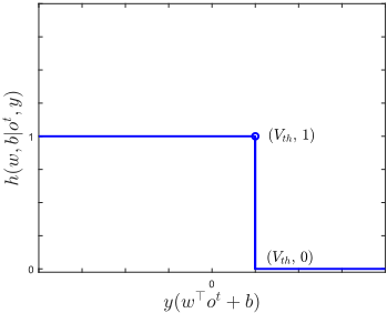
where f(w, b|ot , y) = y(w⊤ot + b), ‖ · ‖0 is the ℓ0-norm, Vth > 0, and (·)+ maps the negative values to 0. Based on Eq. (7) and Fig. 2, if f(w, b|ot , y) < Vth, the output neuron is rest and h(w, b|ot , y) = 1. Otherwise, the neuron fires a spike and h(w, b|ot , y) = 0.
Summarizing all h(w, b|ot , y) from t = 1 to T , we obtain the following Spike Counting Loss (SCL):
It is obvious that the value of SCL (Eq. (8)) is integer and bounded by 0 and T. The smaller H(w, b|{ot }Tt=1 , y), the more spikes for a prediction are fired. Ideally, a correct prediction should fire the spikes at every time step, that is, H(w, b|{ot }Tt=1 , y) = 0, and the spike activities of the negative samples should keep at rest.
Different from Eq. (3), the SCL constrains the prediction of each step to satisfy y(w⊤ot + b) ≥ Vth rather than maximizing a predicted probability or directly fitting the target. Compared to the existing spike-base loss functions, the value of SCL is discreteness.
3.2 Spike Count Maximization
To ensure that SCL activates the output spikes with sufficient confidence. We model the SNN's training problem by combining the structural risk minimization [Vapnik, 2000] with Eq. (8).
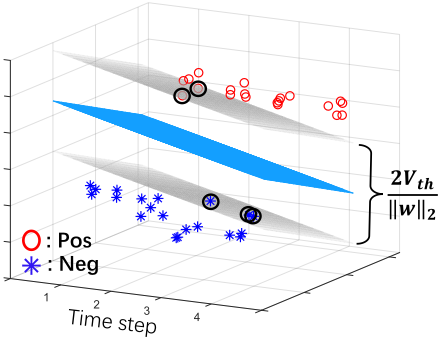
Fig. 3 gives an example of Eq. (9) on spatial-temporal data, which has two dimension features and four inference steps. The blue hyperplanes is the classifier, the gray planes are the margin boundaries of the firing threshold y(w⊤o+b) = Vth. The training of regular term ‖w‖22 maximizes the margin 2Vth ‖w‖2 , which separates positive and negative samples with enough confidence. H(·) minimizes the number of projections located in the negative direction of Vth = y(w⊤o + b) (refer to the data marked by the dashed circles in Fig. 3) and is equivalent to maximize the number of features satisfying y(w⊤ot + b) ≥ Vth, t ∈ [1, T ].
3.3 Iterative Solutions
Since the SCM is a optimization problem that relates to the spike counts, Eq. (9) is a mixed integer programming (MIP) problem. The popular gradient descent can not be applied for the optimization of Eq. (9) since the ℓ0 terms gradient is 0. This section proposes the iterative solutions for Eq. (9).
Given a spatial-temporal feature set {{oti }Tt=1 , yi}Ni=1 with two classes yi ∈ {-1, +1}. The SCL becomes
Let z = [w⊤, b]⊤ denotes the classifier, Xt = [ot1 , ot2 , . . . , otN ], and Y be a diagonal matrix with diag(Y ) = [y1, y2, . . . , yN]. We can reform Eq. (10) to the following equation
where At = Y [(Xt )⊤ 1]. Then, we use g(·) to denote the ℓ0 term
and Eq. (9) is simplified as
where D is a diagonal matrix with diag(D) = [1⊤d , 0]⊤. It is equivalent to the constraint problem:
By replacing Atz with the potential ut and introducing the equality constraint, the optimization of the ℓ0-norm is independent of z, and the objective function of Eq. (14) can be relaxed to
where ρ > 0 and β > 0 are the penalty parameters. We can minimize Eq. (15) to learn the classifier z.
Based on the above analysis, the training of Eq.(9) is decomposed to optimize z and {ut }Tt=1 . Since the optimization of ut is non-differentiable, we minimize Eq. (15) by the block coordinate descent [Tseng, 2001; Tang et al., 2018] and have the following iterative scheme:
where k denotes the k-th training iteration and λ > 0 is a small enough value.
We present the solutions of Eq. (16) in Theorem 1. Compared with the surrogate gradient-based training of the existing spike-based loss functions, Theorem 1 learns the classifier by Eq. (17) and optimizes the output spikes based on Eq. (18).
Theorem 1. The solutions of Eq. (16) are
where at = Atzk+1 - βρ , 1 ≤ i ≤ N, 1 ≤ t ≤ T .
We extend the SCM for multi-class classification by applying the "one-versus-all" strategy:
where C denotes the class number, zc = [w⊤c bc]⊤, and Atc = Y c[(Xt )⊤1]. We solve each class's (zc,utc ) based on Theorem 1.
Algorithm 1 Spike Count Maximization
Input: Training set {{xti }Tt=1 , yi}Ni=1 , number of class: C, time steps: T, Layers of SNN: M, SNN training epoch & loss function: E,L, and SCM iteration: K, parameters: ρ > 0, γ > 0, β ≥ 0.
Parameter: The SNN f(·) with parameters {W m, bm}Mm=1 , Parameters for SCM: {zc, }Cc=1 , {utc }Cc=1 Output: The trained SNN.
- 1: Stage 1: Train the SNN {W m, bm}Mm=1 based on Spike-based gradient algorithm
- 2: Collect the M - 1 layer's features from the SNN: 3: for t = 1 to T do 4: for i = 1 to N do 5: oti = f({W m, bm}M-1 m=1 |xti , yi). 6: end for 7: Xt = [ot1 , ot2 , . . . , otN ]. 8: end for 9: Stage 2: Train the classifier zc by solving Eq. (19). 10: for k = 0 to K do 11: for c = 1 to C do 12: Update zc based on Eq. (17). 13: for t = 1 to T do 14: Update utc based on Eq. (18). 15: end for 16: end for 17: end for 18: Let W = [w1,w2, . . . ,wC], b = [b1, b2, . . . , bC]⊤, where wc = zk+1 c(1:d) , bc = zk+1 cd+1 , 1 ≤ c ≤ C. 19: Replace the decision layer of SNN with W and b: W M = W, bM = b; 20: Return {W m, bm}Mm=1 .
To ensure the convergence of the model, the training pipeline of the SCM is separated into two stages: Stage 1: Pre-train the SNN; Stage 2: Train the classifier zc by solving Eq. (19). For Stage 1, we can apply the popular loss functions to train the SNN. In Stage 2, we extract the spatialtemporal features from the well-trained SNNs and train the classifier by solving Eq. (19). We state the details of the SCM in Algo. 1.
4 Experiments
This section estimates the SCM on the neuromorphic datasets (DVS128-GESTURE, CIFAR10-DVS, and ASL-DVS). We compare our SCM with the SNNs trained based on the popular loss functions and spike-based BP algorithms. Details of the setting and results are presented in the following sections.
4.1 Experiment Setting
Tab.1 shows the neuromorphic datasets: DVS128-GESTURE (DVS-G) [Amir et al., 2017], CIFAR10-DVS (C10-DVS) [Li et al., 2017], and ASL-DVS [Bi et al., 2019] the DVS captures. Before training, we scale the frame size to 32×32×2. Then, we set the time steps T of DVS-G, C10-DVS, and ASLDVS to 40, 20, and 20 by the event-to-frame process [Fang et al., 2020], respectively. For C10-DVS, we randomly separate 90% of the samples for training and 10% for testing.
| Dataset | Frame Size | Categories | Samples | |
|---|---|---|---|---|
| Train Set | Test Set | |||
| DVS128-GESTURE | 128×128×2 | 11 | 1,176 | 288 |
| CIFAR10-DVS | 128 × 128 × 2 | 10 | 10,000 | |
| ASL-DVS | 120 × 240 × 2 | 24 | 211,392 | |
For ASL-DVS, we randomly separate 80% of the samples for training and 20% for testing. The Parametric LIF neurons [Fang et al., 2021b] with Vth = 1 is applied for SNN modeling. For a fair comparison, a ResNet-18 SNN [Fang et al., 2020] (11.17M Params, Conv1:{3 × 3, 64, stride 1}, Conv3 1: {stride 1}) without the max-pooling layer is applied as the backbone for all training approaches. All models share the same training/testing set. We adopt the Adam optimizer with a learning rate of 0.001 to train all models in Stage 1, and the training epochs of DVS-G, C10-DVS, and ASL-DVS are 30, 30, and 3. For Stage 2 training, we set the iterations to 10, β = 0.01, ρ = 1, and γ ranges from 0.001 to 1000 with a step size of 10. The accuracy of all models is predicted by two metrics: a) MP Acc and b) Spike Acc. The MP Acc accumulates the MPs of the last layer for prediction, and the Spike Acc makes predictions by all output spikes. All results are averaged over 5 runs.
4.2 Performance
Comparison With Different Loss Functions
In this part, we compare the SCM with the SNNs supervised by the MP-based loss functions: CE, MSE, and TET [Deng et al., 2022a], and spike-based loss functions: SCE [Wu et al., 2019a; Meng et al., 2022], SRL [Shrestha and Orchard, 2018; Kaiser et al., 2020] with ˆ ryi = 1.0, and SpikeMax [Shrestha et al., 2022]. We use the PiecewiseLeakyReLU function [Wu et al., 2018; Wu et al., 2019b; Fang et al., 2020] as the surrogate gradient to train the SNNs. We initialize the MP-lossbased models by a SNN that is pre-trained on CIFAR100. Then, the spike-loss-based SNNs is initialized by the trained MP-loss-based SNNs. The accuracy results are shown in Tab. 2. Using output spikes for prediction degrades the performance of CE, MSE, and TET-based SNNs. Although the degeneration of the CE loss is lower than that of the MSE and TET, the accuracies are 1.82% and 8.42% lower than the MP Acc on C10-DVS and ASL-DVS, respectively. By applying the SCM to train the classifier of the CE-based SNNs, the Spike Acc on DVS-G, C10-DVS, and ASL-DVS are improved to 96.11%, 77.50%, and 99.23%, respectively.
The SCM improves the MP Acc of models trained with MP-based loss functions, although it does not directly optimize the MP. Both MP Acc and Spike Acc of the spike-based losses outperform the MP-based losses in most cases. Nevertheless, the performance of the MP-based SNNs with SCM is competitive. For C10-DVS, the SNN with "MSE+SCM" performs 1.34% better than the "SRL" on Spike Acc. The SCM also improves the performance of the SCE, SRL, and SpikeMax-based SNNs, with 0.07% ∼ 0.57%, 2.74% ∼ 3.36%, and 0.15% ∼ 0.74% improvements over Spike Acc on DVS-G, C10-DVS, and ASL-DVS, respectively.
| DVS128-GESTURE (T=40) | CIFAR10-DVS (T=20) | ASL-DVS (T=20) | ||||
|---|---|---|---|---|---|---|
| Training Loss | MP Acc (%) | Spike Acc (%) | MP Acc (%) | Spike Acc (%) | MP Acc (%) | Spike Acc (%) |
| CE | 95.28±0.80 | 95.07±0.40 | 75.74±0.89 | 73.92±1.96 | 96.68±4.51 | 88.26±3.99 |
| CE+SCM | 96.04±0.31 | 96.11±0.29 | 78.02±0.86 | 77.50±0.71 | 99.45±0.40 | 99.23±0.65 |
| MSE | 96.18±0.78 | 93.82±1.62 | 76.26±0.48 | 68.96±2.13 | 98.97±1.41 | 75.13±3.03 |
| MSE+SCM | 96.60±1.05 | 96.46±0.89 | 79.06±0.71 | 78.46±0.63 | 99.67±0.22 | 99.55±0.37 |
| TET | 95.28±0.40 | 95.00±0.76 | 75.68±0.99 | 71.48±1.08 | 97.61±2.27 | 79.81±4.46 |
| TET+SCM | 96.04±0.31 | 96.11±0.29 | 77.76±0.58 | 76.98±0.80 | 99.47±0.37 | 99.15±0.72 |
| SCE | 95.97±0.39 | 95.83±0.55 | 77.04±0.89 | 76.64±1.21 | 99.11±0.49 | 98.94±0.50 |
| SCE+SCM | 95.83±0.35 | 95.90±0.29 | 80.16±0.98 | 80.00±0.89 | 99.70±0.12 | 99.68±0.12 |
| SRL | 95.90±0.75 | 96.11±0.67 | 77.32±0.52 | 77.12±0.96 | 99.70±0.17 | 99.64±0.23 |
| SRL+SCM | 96.60±0.75 | 96.68±1.02 | 80.24±0.90 | 79.86±0.65 | 99.83±0.11 | 99.79±0.11 |
| SpikeMax | 96.32±0.53 | 95.83±0.55 | 77.30±0.79 | 76.78±0.62 | 99.47±0.18 | 99.33±0.21 |
| SpikeMax + SCE | 95.97±0.58 | 95.90±0.45 | 80.22±0.85 | 80.12±0.89 | 99.75±0.06 | 99.73±0.06 |
| Gradient Rewriting [Chen et al., 2021] | ||||||
|---|---|---|---|---|---|---|
| DVS128-GESTURE (T=40) | CIFAR10-DVS (T=20) | ASL-DVS (T=20) | ||||
| Training Loss | MP Acc (%) | Spike Acc (%) | MP Acc (%) | Spike Acc (%) | MP Acc (%) | Spike Acc (%) |
| CE CE+SCM | 95.42±0.29 96.18±0.43 | 95.21±0.29 96.25±0.29 | 76.56±0.49 79.28±0.36 | 76.36±0.86 78.48±0.55 | 99.08±0.99 99.60±0.36 | 99.19±0.78 99.60±0.32 |
| MSE MSE+SCM | 94.38±0.52 95.97±0.40 | 93.40±0.55 95.97±0.40 | 76.72±0.65 79.48±0.54 | 71.04±1.59 79.14±0.31 | 99.65±0.24 99.81±0.12 | 86.33±7.29 99.78±0.13 |
| TET TET+SCM | 94.65±0.80 95.76±0.38 | 94.79±0.35 95.97±0.53 | 77.04±0.98 79.66±0.83 | 76.66±0.94 79.24±0.93 | 99.37±0.32 99.75±0.05 | 95.70±1.69 99.60±0.12 |
| Differentiable Spike [Li et al., 2021] | ||||||
| CE CE+SCM | 95.56±0.45 96.18±0.35 | 95.63±0.63 96.39±0.58 | 76.44±0.72 79.14±0.82 | 75.66±1.18 79.12±0.76 | 99.08±0.80 99.73±0.08 | 98.97±0.87 99.71±0.09 |
| MSE MSE+SCM | 94.51±0.38 95.56±0.75 | 90.97±1.30 95.63±0.47 | 77.14±0.43 79.74±0.50 | 62.72±4.07 79.22±0.35 | 99.55±0.28 99.76±0.13 | 81.41±3.30 99.75±0.13 |
| TET | 94.44±0.35 | 94.72±0.52 | 76.02±0.88 | 75.86±1.16 | 99.34±0.34 | 98.14±2.03 |
| TET+SCM | 96.18±0.55 | 96.18±0.49 | 79.74±1.05 | 79.28±1.27 | 99.71±0.10 | 99.59±0.19 |
Comparison With Difference Training Approaches
The surrogate gradient for SNN training is a potential factor affecting performance. To demonstrate that the SCM can adapt to different training approaches, we apply the two recently developed spike-based BP techniques: Gradient Rewiring (GR) [Chen et al., 2021] and Differentiable Spike (DS) [Li et al., 2021] with CE, MSE, and TET for the training of Stage 1. We initialize the models with the MP-lossbased SNNs given in Tab. 2. The experimental results are presented in Tab. 3. Compared to the MP-loss-based SNNs in Tab. 2, both GR and DS improve the Spike Acc of MP-based and Spike-based predictions in many cases. Nevertheless, the performance gap between MP-based and Spike-based predictions is still large, especially for MSE-based SNNs. All models achieve significant improvement by introducing SCM, similar to the SCM-based models in Tab. 2. For the MSEbased SNN with DS, SCM increases the average Spike and MP Acc from 62.72% and 77.14% to 79.22% and 79.74%.
4.3 Robustness &Generalization
The experiments in the following subsections are analyzed based on the C10-DVS, and MP-based prediction. We analyze the robustness and generalization of the SCM in two aspects: a) The improvement of the SCM for the baselines in every epoch; b) The performance of the SCM using different subsets of training samples. We apply the SCM to the spatial-temporal features of the SNNs of Stage 1 in every training epoch and accordingly train the classifiers for predictions. Experiment results are shown in Fig. 4. The training of Stage 1 requires many epochs to improve accuracy performance for classification. However, the SCM performs better than baseline models in every epoch. In early training epochs, the performance of the baselines is weak, but the SCM significantly improves the performance. For example, the average accuracy of the CE-based model in the first epoch is 51.18%, and the SCM increases the baseline accuracy to 62.88%, showing the robustness of the SCM.
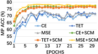
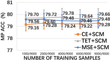
To show the generalization of the SCM, we use the subsets of the C10-DVS with sample numbers given in {1000, 2000, 4000, 6000, 9000} to train the classifier. Experiment results are shown in Fig. 5. By using 1000/9000 sam-
e
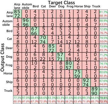
Figure 6: CIFAR10-DVS confusion matrix of the SCM and the MSE-baseline. The last row and column are the recall and precision, respectively. The value in the lower right corner is MP Acc.
ples of the full training set, the SCM improves the accuracy of the GR baseline models from 76.72% (MSE), 76.56% (CE), and 77.04% (TET) to 79.56%, 79.16%, and 79.70%, respectively. We set γ = 0.01, ρ = 1 and apply 1000 training samples for SCM to verify the generalization further. We choose the MSE-based SNN as the baseline for SCM, and the confusion matrix is presented in Fig. 6. For each output class, the first row shows the results of the SCM, and the second row shows the results of the MSE-baseline. The SCM improves the average recall of the MSE-baseline from 73.09% to 79.42%. In addition, the average precision of SCM is 79.34%, while the MSE-baseline is 78.91%. Besides, the accuracy is increased from 73.10% to 79.60%.
4.4 Convergence
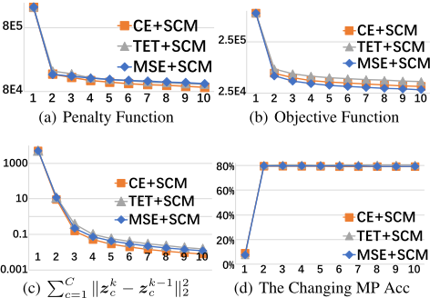
We show the convergence of the SCM based on the changing value of the penalty function, the objective function, the regular term of zc, and the accuracy of each iteration. The baseline models are trained by GR, and the SCM is trained based on ρ = 1, γ = 0.01, and 9000 training samples. The results are shown in Fig. 7. All curves in Fig. 7(a)∼7(c) decrease and converge. The decrease of the penalty function and the regularizer shows the convergence of Eq. (16) and shows that Eq. (9) can be approximated by solving Eq. (15). Based on Fig.7(d), we find that the SCM converges fast, and the best accuracy scores of all models are 79.70% (MSE+SCM), 79.40% (CE+SCM), and 80.50% (TET+SCM).
4.5 Influence of Parameters γ and ρ
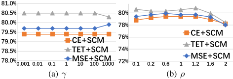
We analyze the influence of γ and ρ based on the accuracy, and the results are given in Fig. 8. We fix ρ = 1 to show the influence of γ. For the analysis of the influence of ρ, we set γ = 0.01. The SCM stays stable in most cases. Based on Fig. 8(a), the fluctuations of all models are small if the γ ranges from 0.001 to 1000. The MSE+SCM, CE+SCM, and TET+SCM achieve 79.90% (γ = 1000), 79.40% (γ ≤ 1000), and 80.50% (γ < 1000), respectively. As shown in Fig. 8(b), all models keep stability if ρ < 2. By setting ρ = 1.2, the SCM+TET achieves 80.80% accuracy performance.
5 Conclusions
In this paper, we propose the SCM to train the SNN by optimizing the output spikes. We propose the spike counting loss to count the output spikes and design the two-stage algorithm for training. Experimental results on various neuromorphic datasets demonstrate the effectiveness of the SCM. Since the matrix multiplication complexity of the Stage 2 is proportional to the number of samples, the SCM is inefficient on large datasets. In addition, the two-stage strategy may be suboptimal for the SCM because the backbone is fixed to extract features for the Stage 2 training. Our future work will focus on improving the efficiency of the SCM.
Acknowledgements
This work was supported in part by the Key-Area Research and Development Program of Guangzhou (202007030004); in part by the National Natural Science Foundation of China (62076258).
@inproceedings{ijcai2023p473,
  title     = {Spike Count Maximization for Neuromorphic Vision Recognition},
  author    = {Tang, Jianxiong and Lai, Jian-Huang and Xie, Xiaohua and Yang, Lingxiao},
  booktitle = {Proceedings of the Thirty-Second International Joint Conference on
               Artificial Intelligence, {IJCAI-23}},
  publisher = {International Joint Conferences on Artificial Intelligence Organization},
  editor    = {Edith Elkind},
  pages     = {4253--4261},
  year      = {2023},
  month     = {8},
  note      = {Main Track},
  doi       = {10.24963/ijcai.2023/473},
  url       = {https://doi.org/10.24963/ijcai.2023/473},
}
TY - CPAPER TI - Spike Count Maximization for Neuromorphic Vision Recognition AU - Tang, Jianxiong AU - Lai, Jian-Huang AU - Xie, Xiaohua AU - Yang, Lingxiao T2 - Proceedings of the Thirty-Second International Joint Conference on Artificial Intelligence, IJCAI-23 PB - International Joint Conferences on Artificial Intelligence Organization PY - 2023 SP - 4253 EP - 4261 DO - 10.24963/ijcai.2023/473 UR - https://doi.org/10.24963/ijcai.2023/473 ER -Copied
Machine-readable versions of this paper, for tools and AI agents:





