
Context-Aware Feature Selection and Classification
Proceedings of the Thirty-Second International Joint Conference on Artificial Intelligence. Main Track. Pages 4317-4325.
https://doi.org/10.24963/ijcai.2023/480
Keywords
- Machine Learning: ML: Feature extraction, selection and dimensionality reduction
- Machine Learning: ML: Classification
- Machine Learning: ML: Explainable/Interpretable machine learning
Abstract
We propose a joint model that performs instance-level feature selection and classification. For a given case, the joint model first skims the full feature vector, decides which features are relevant for that case, and makes a classification decision using only the selected features, resulting in compact, interpretable, and case-specific classification decisions. Because the selected features depend on the case at hand, we refer to this approach as context-aware feature selection and classification. The model can be trained on instances that are annotated by experts with both class labels and instance-level feature selections, so it can select instance-level features that humans would use. Experiments on several datasets demonstrate that the proposed model outperforms eight baselines on a combined classification and feature selection measure, and is able to better emulate the ground-truth instance-level feature selections. The supplementary materials are available at https://github.com/IIT-ML/IJCAI23-CFSC.
- [Adriaenssens et al., 2004] Veronique Adriaenssens, Bernard De Baets, Peter LM Goethals, and Niels De Pauw. Fuzzy rule-based models for decision support in ecosystem management. Science of the Total Environment, 319(1-3):1-12, 2004.
- [Arai et al., 2016] Hiromasa Arai, Crystal Maung, Ke Xu, and Haim Schweitzer. Unsupervised feature selection by heuristic search with provable bounds on suboptimality. In Thirtieth AAAI Conference on Artificial Intelligence, 2016.
- [Arya et al., 2019] Vijay Arya, Rachel KE Bellamy, Pin-Yu Chen, Amit Dhurandhar, Michael Hind, Samuel C Hoff- man, Stephanie Houde, Q Vera Liao, Ronny Luss, Alek- sandra Mojsilović, et al. One explanation does not fit all: A toolkit and taxonomy of ai explainability techniques. arXiv preprint arXiv:1909.03012, 2019.
- [Bahdanau et al., 2014] Dzmitry Bahdanau, Kyunghyun Cho, and Yoshua Bengio. Neural machine translation by jointly learning to align and translate. arXiv preprint arXiv:1409.0473, 2014.
- [Barrett et al., 2018] Maria Barrett, Joachim Bingel, Nora Hollenstein, Marek Rei, and Anders Søgaard. Sequence classification with human attention. In Proceedings of the 22nd Conference on Computational Natural Language Learning, pages 302-312, 2018.
- [Bastings and Filippova, 2020] Jasmijn Bastings and Katja Filippova. The elephant in the interpretability room: Why use attention as explanation when we have saliency meth- ods? arXiv preprint arXiv:2010.05607, 2020.
- [CDC, 2017] CDC. National health interview survey (nhis) dataset. https://www.cdc.gov/nchs/nhis/nhis 2017 data release.htm, 2017. Accessed: 2023-01-14. Link
- [City of Chicago, 2019] City of Chicago. Ride-sharing dataset. https://data.cityofchicago.org/Transportation/ Transportation-Network-Providers-Trips-2019/ iu3g-qa69, 2019. Accessed: 2023-01-14. Link
- [Cohen, 1995] William W Cohen. Fast effective rule induc- tion. In Machine learning proceedings 1995, pages 115- 123. Elsevier, 1995.
- [Das et al., 2013] Shubhomoy Das, Travis Moore, Weng- Keen Wong, Simone Stumpf, Ian Oberst, Kevin McIn- tosh, and Margaret Burnett. End-user feature label- ing: Supervised and semi-supervised approaches based on locally-weighted logistic regression. Artificial Intelli- gence, 204:56-74, 2013.
- [De Laat, 2018] Paul B De Laat. Algorithmic decision- making based on machine learning from big data: can transparency restore accountability? Philosophy & tech- nology, 31(4):525-541, 2018.
- [Fürnkranz and Widmer, 1994] Johannes Fürnkranz and Gerhard Widmer. Incremental reduced error pruning. In Machine Learning Proceedings 1994, pages 70-77. Elsevier, 1994.
- [Gao et al., 2016] Shuyang Gao, Greg Ver Steeg, and Aram Galstyan. Variational information maximization for fea- ture selection. arXiv preprint arXiv:1606.02827, 2016.
- [Ghaeini et al., 2018] Reza Ghaeini, Xiaoli Z Fern, and Prasad Tadepalli. Interpreting recurrent and attention- based neural models: a case study on natural language in- ference. arXiv preprint arXiv:1808.03894, 2018.
- [Goyal, 2020] Goyal. Credit card customers dataset. https://www.kaggle.com/datasets/sakshigoyal7/ credit-card-customers, 2020. Accessed: 2022-08-13. Link
- [Guidotti, 2021] Riccardo Guidotti. Evaluating local expla- nation methods on ground truth. Artificial Intelligence, 291:103428, 2021.
- [Hall, 2000] Mark A Hall. Correlation-based feature selec- tion for discrete and numeric class machine learning. In Proceedings of the Seventeenth International Conference on Machine Learning, pages 359-366, 2000.
- [Harradon et al., 2018] Michael Harradon, Jeff Druce, and Brian Ruttenberg. Causal learning and explanation of deep neural networks via autoencoded activations. arXiv preprint arXiv:1802.00541, 2018.
- [Holte, 1993] Robert C Holte. Very simple classification rules perform well on most commonly used datasets. Ma- chine learning, 11(1):63-90, 1993.
- [Jain and Wallace, 2019] Sarthak Jain and Byron C Wal- lace. Attention is not explanation. arXiv preprint arXiv:1902.10186, 2019.
- [Jang et al., 2016] Eric Jang, Shixiang Gu, and Ben Poole. Categorical reparameterization with gumbel-softmax. arXiv preprint arXiv:1611.01144, 2016.
- [Kohavi and John, 1997] Ron Kohavi and George H John. Wrappers for feature subset selection. Artificial intelli- gence, 97(1-2):273-324, 1997.
- [Lage et al., 2019] Isaac Lage, Emily Chen, Jeffrey He, Menaka Narayanan, Been Kim, Sam Gersh- man, and Finale Doshi-Velez. An evaluation of the human-interpretability of explanation. arXiv preprint arXiv:1902.00006, 2019.
- [Lei et al., 2016] Tao Lei, Regina Barzilay, and Tommi Jaakkola. Rationalizing neural predictions. In Proceed- ings of the 2016 Conference on Empirical Methods in Nat- ural Language Processing, pages 107-117, Austin, Texas, November 2016. Association for Computational Linguis- tics.
- [Lei et al., 2020] Wenqiang Lei, Xiangnan He, Yisong Miao, Qingyun Wu, Richang Hong, Min-Yen Kan, and Tat-Seng Chua. Estimation-action-reflection: Towards deep interac- tion between conversational and recommender systems. In Proceedings of the 13th International Conference on Web Search and Data Mining, pages 304-312, 2020.
- [Letham et al., 2015] Benjamin Letham, Cynthia Rudin, Tyler H McCormick, and David Madigan. Interpretable classifiers using rules and bayesian analysis: Building a better stroke prediction model. The Annals of Applied Statistics, 9(3):1350-1371, 2015.
- [Li et al., 2015] Jiwei Li, Xinlei Chen, Eduard Hovy, and Dan Jurafsky. Visualizing and understanding neural mod- els in nlp. arXiv preprint arXiv:1506.01066, 2015.
- [Li et al., 2019] Chaoqun Li, Liangxiao Jiang, and Wen- qiang Xu. Noise correction to improve data and model quality for crowdsourcing. Engineering Applications of Artificial Intelligence, 82:184-191, 2019.
- [Lundberg and Lee, 2017] Scott M Lundberg and Su-In Lee. A unified approach to interpreting model predictions. In Proceedings of the 31st international conference on neural information processing systems, pages 4768-4777, 2017.
- [Martins and Astudillo, 2016] Andre Martins and Ramon Astudillo. From softmax to sparsemax: A sparse model of attention and multi-label classification. In Interna- tional conference on machine learning, pages 1614-1623.
- PMLR, 2016.
- [Melville and Sindhwani, 2009] Prem Melville and Vikas Sindhwani. Active dual supervision: Reducing the cost of annotating examples and features. In Proceedings of the NAACL HLT 2009 workshop on active learning for natu- ral language processing, pages 49-57, 2009.
- [Moeyersoms et al., 2016] Julie Moeyersoms, Brian d'Alessandro, Foster Provost, and David Martens. Ex- plaining classification models built on high-dimensional sparse data. arXiv preprint arXiv:1607.06280, 2016.
- [Molnar, 2020] Christoph Molnar. Interpretable machine learning. Lulu. com, 2020.
- [Narendra et al., 2018] Tanmayee Narendra, Anush Sankaran, Deepak Vijaykeerthy, and Senthil Mani. Explaining deep learning models using causal inference. arXiv preprint arXiv:1811.04376, 2018.
- [Purohit et al., 2012] Seema U Purohit, Venkatesh Mahade- van, and Anjali N Kulkarni. Credit evaluation model of loan proposals for indian banks. International Journal of Modeling and Optimization, 2(4):529-534, 2012.
- [Ribeiro et al., 2016] Marco Tulio Ribeiro, Sameer Singh, and Carlos Guestrin. " why should i trust you?" explain- ing the predictions of any classifier. In Proceedings of the 22nd ACM SIGKDD international conference on knowl- edge discovery and data mining, pages 1135-1144, 2016.
- [Ribeiro et al., 2018] Marco Tulio Ribeiro, Sameer Singh, and Carlos Guestrin. Anchors: high-precision model- agnostic explanations. In Proceedings of the Thirty- Second AAAI Conference on Artificial Intelligence and Thirtieth Innovative Applications of Artificial Intelligence Conference and Eighth AAAI Symposium on Educational Advances in Artificial Intelligence, pages 1527-1535, 2018.
- [Seerat and Qamar, 2015] Bakhtawar Seerat and Usman Qa- mar. Rule induction using enhanced ripper algorithm for clinical decision support system. In 2015 Sixth Interna- tional Conference on Intelligent Control and Information Processing (ICICIP), pages 83-91. IEEE, 2015.
- [Serrano and Smith, 2019] Sofia Serrano and Noah A Smith. Is attention interpretable? arXiv preprint arXiv:1906.03731, 2019.
- [Sharma and Bilgic, 2018] Manali Sharma and Mustafa Bil- gic. Learning with rationales for document classification. Machine Learning, 107(5):797-824, 2018.
- [Sharma, 2017] Sharma. Mobile price dataset. https://www.kaggle.com/datasets/iabhishekofficial/ mobile-price-classification, 2017. Accessed: 2022-08-13. Link
- [Shrestha et al., 2019] Yash Raj Shrestha, Shiko M Ben- Menahem, and Georg Von Krogh. Organizational decision-making structures in the age of artificial intel- ligence. California Management Review, 61(4):66-83, 2019.
- [Tanno et al., 2019] Ryutaro Tanno, Ardavan Saeedi, Swami Sankaranarayanan, Daniel C Alexander, and Nathan Sil- berman. Learning from noisy labels by regularized es- timation of annotator confusion. In Proceedings of the IEEE/CVF conference on computer vision and pattern recognition, pages 11244-11253, 2019.
- [Wachter et al., 2017] Sandra Wachter, Brent Mittelstadt, and Chris Russell. Counterfactual explanations without opening the black box: Automated decisions and the gdpr. Harv. JL & Tech., 31:841, 2017.
- [Wang et al., 2016] Yequan Wang, Minlie Huang, Xiaoyan Zhu, and Li Zhao. Attention-based lstm for aspect-level sentiment classification. In Proceedings of the 2016 con- ference on empirical methods in natural language process- ing, pages 606-615, 2016.
- [Wang et al., 2022] Juanyan Wang, Manali Sharma, and Mustafa Bilgic. Ranking-constrained learning with ratio- nales for text classification. In Findings of the Association for Computational Linguistics: ACL 2022, pages 2034- 2046, 2022.
- [Yu and Liu, 2003] Lei Yu and Huan Liu. Feature selection for high-dimensional data: A fast correlation-based filter solution. In Proceedings of the 20th international con- ference on machine learning (ICML-03), pages 856-863, 2003.
- [Zaidan et al., 2007] Omar Zaidan, Jason Eisner, and Chris- tine Piatko. Using "annotator rationales" to improve ma- chine learning for text categorization. In Human language technologies 2007: The conference of the North American chapter of the association for computational linguistics; proceedings of the main conference, pages 260-267, 2007.
- [Zhang et al., 2016] Ye Zhang, Iain Marshall, and Byron C Wallace. Rationale-augmented convolutional neural net- works for text classification. In Proceedings of the Confer- ence on Empirical Methods in Natural Language Process- ing. Conference on Empirical Methods in Natural Lan- guage Processing, volume 2016, page 795. NIH Public Access, 2016.
- [Zieba et al., 2016] Maciej Zieba, Sebastian K Tomczak, and Jakub M Tomczak. Ensemble boosted trees with synthetic features generation in application to bankruptcy predic- tion. Expert systems with applications, 58:93-101, 2016.
References were extracted automatically from the PDF and may contain errors.
Full text extracted automatically from the PDF; figures, tables and equations may differ. The PDF is the version of record.
1 Introduction
A barrier to using highly accurate machine learning algorithms for decision support is their opacity [De Laat, 2018]. While opacity might be acceptable for certain tasks, such as handwritten digit recognition, when machine learning systems are used to assist humans in decision making, the algorithms must be able to explain their decision making processes and these explanations need to make sense to humans in order to be useful. For instance, when a machine learning system is employed for loan decisions, the reasons for approving or rejecting a loan must be explained in a humanunderstandable form to the loan officer (who will make the final decision based on the system's recommendations and explanations), to the applicant (who is directly impacted by the decision), to the developer (for debugging), and to the regulators (to ensure the system's decisions are not discriminatory) [Arya et al., 2019].
While being interpretable and able to explain its decisions are important and necessary, they are not sufficient for a model to be effective in a decision support system. For example, a logistic regression model is assumed to be interpretable. However, when the model uses thousands of features, the explanations are rarely useful as inspecting the relative impact of all relevant features will be overwhelming for the stakeholders (decision makers, users, etc.). Likewise, a decision tree, while considered interpretable, is not necessarily useful for decision support. One can impose sparsity, such as using L1 regularization for logistic regression, or a depth limit on the decision tree. While sparsity can make the models simpler, it often does so by prioritizing common features that have the greatest impact on the most number of objects (e.g., the word 'movie' tends to be a common and a statistically negative term in a movie review classification task), which may not be the most meaningful features for stakeholders [Lage et al., 2019].
Additionally, when people make decisions, they tend to quickly scan all available information and then focus on few factors that are relevant for the case at hand [Shrestha et al., 2019]. For instance, when loan officers review a loan application, they skim the entire application and then focus on what is relevant for the case. While all information is used, the income and the credit score might be the determining factors for one application while the number of missed payments might be the determining factor for another [Purohit et al., 2012]. The human decision maker is essentially performing what we call context-aware feature selection and classification: skimming the full feature set, focusing on the features that are relevant for the current case, and making a classification decision using only the selected features.
Context-aware feature selection by machine learning models is limited. Traditional feature selection methods such as L1 regularization and filter methods perform 'global' feature selection where the same set of features are used for all objects, as opposed to context-aware feature selection where the selected features depend on the object itself. While decision trees perform context-aware feature selection, the rules provided by decision trees are hierarchical, and hence some features, like the root and the features close to the root, will repeatedly be selected. They are also not necessarily accurate in learning the complex relationships between data points and features. Rule-based systems perform context-based feature selection, but they also tend to have low accuracy [Molnar, 2020]. Attention-based neural networks [Bahdanau et al., 2014] can perform context-aware feature selection and be highly accurate. However, the selected features are not guaranteed to be meaningful to humans. We discuss related work in more detail in the next section.
When explanations that are meaningful to humans are desired, one approach is to ask for supervision from humans on which features they focused for each classification decision. We refer to these as instance-level feature labels, as opposed to global feature labeling [Melville and Sindhwani, 2009; Das et al., 2013]. Eliciting instance-level features from humans requires extra time, effort, and cost; hence, instancelevel feature labeling is practical for only domains where human-like explanations and decisions are desired. We experiment with both fully-automated baselines that do not need instance-level feature labels as well as with the ones that can use them if available.
Our contributions in this paper include:
- We introduce and formalize the context-aware feature selection and classification problem.
- We propose a context-aware feature selection and classification model that jointly utilizes class labels and instance-level feature selection annotations.
- We conduct experiments to empirically compare the proposed model to a number of baselines on several datasets, comparing them using both classification performance and feature selection performance.
The rest of the paper is organized as follows. We discuss related work in the next section. We present our model in Section 3. We discuss the experimental methodology in Section 4. We discuss our findings in Section 5 and followed by a discussion of limitations in Section 6, and then conclude.
2 RelatedWork
2.1 Feature Selection
Traditional feature selection methods can be broadly categorized into three: i) filter methods use a feature importance measure such as feature correlation [Hall, 2000; Yu and Liu, 2003] and mutual information [Gao et al., 2016], to rank and select features; ii) wrapper methods that iteratively search for the best set of features for a given model [Kohavi and John, 1997; Arai et al., 2016]; iii) and, methods that embed the feature selection into the learning process, such as decision trees, rule-based systems, and L1-regularized models. We used decision tree and L1 regularized logistic regression as two baselines in our experiments.
2.2 Rule-Based Systems
Rule-based systems have been extensively used for decision support [Adriaenssens et al., 2004; Seerat and Qamar, 2015]. They were preferred for their interpretability. Approaches include OneR that created rules with one feature [Holte, 1993], IREP that used a combination of pre-pruning and postpruning [F¨urnkranz and Widmer, 1994], RIPPER that used rule pruning to optimize the rule set in a post-processing phase [Cohen, 1995], and Bayesian Rule Lists [Letham et al., 2015]. We used RIPPER as a baseline in our experiments.
2.3 Learning with Rationales
A closely related area is learning with rationales which asks annotators to highlight segments of the text per document as 'rationales' for their labeling decisions. Zaidan et al. [2007] converted the rationales into constraints for training support vector machines. Sharma and Bilgic [2018] presented a method to manipulate feature weights in the training of off-the-shelf classifiers. Recent deep learningbased approaches on incorporating rationales either generated rationale-augmented representations of text [Zhang et al., 2016] or utilized the rationales for richer supervision [Barrett et al., 2018; Wang et al., 2022]. Although the main purpose of these methods was to improve classification performance, instead of performing feature selection, some of them can be adapted to perform context-aware feature selection. We adapted Barrett et al. [2018]'s BiLSTM-based method as one of the baselines.
2.4 Model Interpretability
Several papers worked on generating explanations for complex or black-box models. For example, Ribeiro et al. [2016] replaced the underlying complex model with a surrogate model, Lundberg and Lee [2017] computed Shapley values as feature importance, Wachter et al. [2017] used examples for explanations, Li et al. [2015] computed input saliency for neural networks. Our approach differs from most of these post-processing methods as it selects case-specific features that are certainly used by the model for predicting a specific instance. While several papers used attention mechanism for interpretability [Wang et al., 2016; Ghaeini et al., 2018], other papers pointed out that attention weights often reflect how much the model attend to the hidden representation of each input, which might already have mixed in information from other inputs [Bastings and Filippova, 2020], and are not stable indicators for interpretability [Jain and Wallace, 2019; Serrano and Smith, 2019].
Several papers also incorporated interpretability into the approach itself. For example, rationalized neural network [Lei et al., 2016] and causality-based approaches [Narendra et al., 2018; Harradon et al., 2018]. Closest to our task is rationalized neural network [Lei et al., 2016]; they extracted short and continuous 'rationales' from each document for classifying and rationalizing the document. We adapted this approach as a baseline in our experiments.
3 Context-Aware Feature Selection and Classification (CFSC)
We are given a dataset D whose members are triplets ⟨xi, yi, ai⟩ where xi ∈ Rm is an m dimensional input vector, yi ∈ {c1, c2, ..., cq} is a discrete variable representing xi's class label, and ai ∈ {0, 1}m is xi's feature label indicating which features are used by a human in making the classification decision yi for the instance xi.
The objective is to train a model f : xi → ⟨yi, ai⟩ that can generalize to unseen data points xj and correctly predict both the label yj and the feature selections aj for xj. Predicting aj is equivalent to solving a multi-label classification problem as each entry indicates if feature k is selected, ajk ∈ {0, 1}. Note that while f has access to the full triplet ⟨xi, yi, ai⟩ during training time, f has access to only xj at test time and not aj. Hence, at test time f must predict both aj and yj. We refer to this task as a context-aware feature selection and classification problem. The step of predicting aj is the context-aware feature selection where the feature selection decisions, aj , depend on the particular instance xj , as opposed to global feature selection methods. Moreover, to ensure sparsity and interpretability, we require the predicted aj to have exactly 0 for features that are not selected for predicting yj of xj , and the step of predicting yj should use only the selected features.
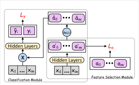
We propose the neural network model depicted in Figure 1 and refer to it as Context-aware Feature Selection and Classification, or CFSC in short. The model contains a contextaware feature selection module and a classification module. It is first trained to predict ai using xi, without initially worrying about yi, and then fine-tuned to predict ai and yi jointly.
The feature selection module processes the input xi through an optional number of hidden layers. The hidden layer part of this module can be as simple or complicated as needed, such as a simple fully-connected dense layer, or a deep neural network consisting of self-attention and dense layers. The output of this process is a′i . a′i are not constrained to be between 0 or 1 and they are not constrained to be sparse just yet, as sparsity will be imposed in the next step. Hence, we use the identity activation at these nodes at this stage.
To train the feature selection module using humanprovided triplets D = {⟨xi, yi, ai⟩}, we formulate the objective as a multi-label classification task. First, we pass each a′ik through a sigmoid of the form 1/(1+ e-a′ik). The weights of the feature selection module, Wa, are then trained using binary cross entropy loss. Let this loss be La. This training process imposes that for a feature that should be selected, i.e., for aik = 1, the a′ik needs to be positive, and a′ik needs to be negative for features where the ground truth is aik = 0.
For predicting yi, we need to use only the features that are selected by the feature selection module. Because the output of the feature module, a′ik , are real-valued, where a′ik > 0 indicates if a feature should be selected, we pass the a′i vector through a ReLU function. That is, ˆai = ReLU(a′i ), guaranteeing that features for which a′ik < 0 will have exactly zero values and ˆai acts as a mask function, performing feature selection.
xi is first multiplied with the predicted feature mask ˆai, xi ⊗ ˆai, which is then passed through a number of optional hidden layers and then used for predicting yi. This overall process is meant to mimic the human decision-making process where the full feature vector xi is first skimmed to decide which features are relevant for the case at hand (ˆai), and only those feature values (xi ⊗ ˆai) are used for predicting yi. Cross entropy is used as the classification loss using the predicted ¯ yi and the ground truth yi. Let this loss be Ly. The overall loss L is a weighted combination of Ly and La:
where λa is the weight of the feature loss. The weights of feature selection module, Wa, are trained to optimize La first, and then the weights of the full model, W=Wa ∪Wy, are jointly trained to optimize the combined loss L.
4 Experimental Methodology
We conduct experiments to compare the proposed CFSC method to several baselines on both classification and feature selection performance. In this section, we describe the baselines, the datasets, the two simulated experts, the combined classification and feature selection measure, the density measure, and the parameter settings.
4.1 Baselines
To the best of our knowledge, no existing paper directly addresses the context-aware feature selection and classification problem for tabular data, except decision trees and rule-based systems. However, several approaches can be adapted to perform this task. We modified and experimented with an attention-based BiLSTMmodel [Barrett et al., 2018], a rationalized neural network [Lei et al., 2016], a pipeline model, and a global feature selection model.
Attention-based Bi-directional LSTM(ATT-FL). This is the main baseline that is closest to our approach and utilizes both ai and yi during training. This baseline is based on the method by Barrett et al. [2018] for text classification. They regularized the attention layer of a Bi-directional LSTM model using 'estimated' human attention from an eye tracking corpora. We adapted their method to be used for vectorbased data as follows: each instance xi is passed through a hidden layer, followed by a Bi-LSTM layer, an attention layer, and finally the classification layer. The softmax in the attention layer is replaced with sparsemax [Martins and Astudillo, 2016] to ensure sparsity and enable feature selection. We refer to this method as ATT-FL. For comparison and to evaluate how much the human-provided feature labels help, we also present results with the fully-automated version of this method that still performs context-aware feature selection but does not need feature labels; we refer to this as ATT.
Rationalizing Neural Predictions (RNP). This method is based on the work of Lei et al. [2016]. It used a generator to extract short and continuous 'rationales' for text classification, where rationales are pieces of text from the document for classifying the document. We adapted this method to a vector-based domain as follows: each instance xi is passed through a generator consisting of two hidden layers and one output layer for rationale selection first. The selected features pass through an encoder consisting of one hidden layer and one output layer for classification. Following the implementation of Lei et al. [2016], we used gumbel-softmax activation function [Jang et al., 2016] coupled with L1 penalty for rationales in the loss function to impose sparsity.
Logistic Regression Pipeline (LR-PL). In contrast to our joint learning approach, one simple baseline is to build a pipeline where one logistic regression model is trained for feature selection and another logistic regression model is trained for classification separately. The first model is trained to perform f1 : xi → ai. The second model is trained to perform f2 : xi ⊗ ¯ai → yi where ¯ai is the predicted binarized feature labels. At test time, f1 is used to predict xj → aj and then f2 is used to predict xj ⊗ ¯aj → yj .
We also experimented with three classification algorithms that simultaneously perform feature selection. A decision tree classifier (DT), a rule-based learner (RL) based on RIPPER [Cohen, 1995](we trained two rule-based learners for binary classification: one aimed at predicting the positive class as RL-P and the other for the negative class as RL-N), and a L1-regularized logistic regression model (LR). Decision tree classifier and rule-based learner perform context-aware feature selection, whereas the L1-regularized logistic regression model performs global feature selection. Finally, we include a feed-forward neural network (FF) that acts as a baseline for only the classification performance.
4.2 Datasets
We experimented with five real-world and three synthetic datasets. The Credit [Goyal, 2020] dataset contains 3,254 bank credit card customers with 37 features and binary labels indicating if the customer is an 'Attrited Customer.' The Company [Zieba et al., 2016] dataset has 4,182 companies with 64 features and binary labels indicating whether the company bankrupted within the forecasting period. The Mobile [Sharma, 2017] dataset contains 2,000 mobile phone data with 20 features and binary labels indicating if the price of a phone is in the high cost range. The NHIS [CDC, 2017] dataset has 2,306 adult survey data with 144 features and binary labels indicating if the person is suffering from chronic obstructive pulmonary disease. The Ride [City of Chicago, 2019] dataset has 4,800 ride trip records with 46 features and binary labels indicating if the trip is shared with other persons. We chose these real-world datasets because the domains are relatively easy for the laypeople, as opposed to more specialized domains. These datasets did not contain instance-level feature labels. Hence, similar to work on generating synthetic explanations [Ribeiro et al., 2018; Guidotti, 2021], we created simulated experts, which we discuss in detail in the next subsection.
We created three synthetic datasets containing instancelevel feature labels where the first two are for binary classification and the third one is a multi-class classification task. We first generated the input data by allocating each class a normally-distributed cluster of points. We trained a shallow decision tree based on the original data and then reassigned class labels based on the predictions of the decision tree. Synthetic1 contains 1,000 instances with 5 features whereas Synthetic2 contains 1,500 instances with 10 features. Synthetic3 contains 3,024 instances with 20 features and four classes. For each xi, the aik is 1 for the features used in the decision path, and 0 otherwise. To experiment with the datasets with different settings, we kept the root node in the decision path and hence one feature was always 'on' for Synthetic1 and Synthetic3 datasets, whereas for Synthetic2 dataset, we removed the root node from the decision path and hence no feature was always 'on.'
4.3 Simulated Expert
We used two strategies to simulate experts that can provide instance-level feature labels. The first strategy is based on the evidence counterfactual method [Moeyersoms et al., 2016]. A logistic regression model is trained on a given dataset. For object xi, let the predicted label be y and wyk be the coefficient of feature k for class y. Starting with the least important feature for xi (i.e., the feature that has the lowest |wyk×xik|), features are removed one by one until the predicted label changes. The top features, including the last one that caused a label flip, are retained as the justification of the classification decision. Because features are ranked by |wyk ×xik| and not simply by |wyk|, this process performs context-aware feature selection, rather than global feature selection.
The second strategy uses a decision tree to generate the instance-level feature labels. First, a decision tree on a given dataset is trained. Then, at prediction time, the features that are used in the decision path for classifying xj are marked as 'on' and the rest are marked as 'off.'
4.4 EvaluationMeasures
One can use traditional evaluation measures, such as accuracy and F1, to evaluate the classification performance. To evaluate the performance of the context-aware feature selection, which is a multi-label classification task, measures such as hamming loss and subset accuracy can be used. However, these measures are crude and inadequate for transparency purposes; while some features are frequently used, others are never used, and some are used rarely. Summarizing everything up in a single measure would not portray the whole picture. Therefore, we introduce a more granular evaluation approach for evaluating context-aware feature selection.
Let T be the evaluation set, Aon δ be the features that are used for all instances in T : Aon δ = {k | aik = 1 for ∀xi ∈ T }, and Aoff δ be the set of features that are never used for any of the objects: Aoff δ = {k | aik = 0 for ∀xi ∈ T }. Let Aν represent the rest of the features, i.e., the features that are used for some objects but not for others. We use accuracy separately for the features in Aon δ and for features in Aoff δ . For features in Aν, however, because the groundtruth aj tend to be sparse for human-interpretable decisions, a measure for imbalanced classes, such as F1, is more appropriate. For feature k ∈ Aν we first calculate F1k, and take a weighted average as F1w, where each F1k is weighted based on the frequency the feature k is 'on.'
In addition to individual classification and feature selection measures, we also present a linear combination of the two:
where ¯a is the binarized ˆa, Ma(a, ¯a) refers to the evaluation of the context-aware feature selection, andMy(y, ¯ y) refers to the evaluation of the classification decisions, and γa controls the relative importance of the feature selection measure.
Finally, we introduce a new measure aimed at understanding how 'dense' each context-aware classification decision is. We calculate the number of features used per instance, on average, in a given dataset:
As an example, assume a domain with 20 features, that there are 100 instances in the evaluation set, and the model uses 2 features for classifying 50 instances, 3 features for 25 instances, 4 features for 15 instances, and 5 features for the remaining 10 instances. The density for such a model would be (50 × 2 + 25 × 3 + 15 × 4 + 10 × 5)/100 = 2.85.
4.5 Model Structures and Parameter Settings
CFSC has one hidden layer with 16 units for the classification module and two hidden layers with 64 and 256 units respectively for the feature selection module. The ATT-FL model has one hidden layer with 64, one BiLSTM layer with 32, and one attention layer with 256 units. The RNP model has one hidden layer with 16 units for the classification module and two hidden layers with 64 and 256 units respectively for the feature selection module. The FF model has one hidden layer with 16 units. We used the same structures for all datasets and did not perform structure search.
Hyper-Parameter Tuning. For each dataset, we use 1/3 of the data as the test set and perform 5-fold validation on the rest of the data where one fold is used for validation and four folds are used for training. We set γa to 0.5 (Equation 2) for all models 1 . We performed grid search with cross validation to optimize all the other tunable hyper-parameters of each method using the combined measure on the validation set. We provide the range of all tunable parameters for each method in the supplementary materials for reproducibility.
5 Results
We first compare CFSC to the baselines on a combined classification and feature selection measure 2 . Then, we conduct a deep dive analysis of the instance-level feature selection of three methods. Finally, we conduct an ablation study to investigate different parameter settings for γa and λa.
5.1 Combined Performance Measures
Tables 1 and 2 present the combined classification F1 and feature selection F1 on eight datasets under the counterfactual and decision-tree expert strategies respectively. All experimental results are reported by taking an average over five different runs, computed over the five-fold validation splits. We compare CFSC with all baselines using the combined measures computed by Equation 2, with γa = 0.5, which balances equally between the F1 for classification and the weighted F1w for feature selection. Note that CFSC and all the baselines except FF tuned their hyper-parameters to maximize the equally-balanced and combined measures.
1 We provide an ablation study of varying γa in Section 5.3.
2 The separate results for classification and feature selection are included in the supplementary materials.
| FF | LR | DT | RL-P | RL-N | ATT | RNP | LR-PL | ATT-FL | CFSC | |
|---|---|---|---|---|---|---|---|---|---|---|
| Credit | .707 | .680 | .701 | .576 | .538 | .549 | .675 | .622 | .745 | .785 |
| Company | .589 | .480 | .456 | .174 | .336 | .506 | .567 | .328 | .608 | .701 |
| Mobile | .853 | .852 | .852 | .716 | .715 | .779 | .842 | .785 | .903 | .907 |
| NHIS | .606 | .598 | .500 | .448 | .477 | .497 | .550 | .685 | .596 | .781 |
| Ride | .679 | .675 | .671 | .492 | .540 | .591 | .659 | .573 | .706 | .765 |
| FF | LR | RL-P | RL-N | ATT | RNP | LR-PL | ATT-FL | CFSC | |
|---|---|---|---|---|---|---|---|---|---|
| Credit | .796 | .772 | .609 | .626 | .631 | .802 | .868 | .829 | .945 |
| Company | .860 | .751 | .170 | .335 | .769 | .808 | .806 | .821 | .895 |
| Mobile | .625 | .624 | .654 | .673 | .524 | .620 | .454 | .601 | .903 |
| NHIS | .758 | .754 | .421 | .538 | .517 | .753 | .905 | .602 | .909 |
| Ride | .787 | .786 | .504 | .625 | .696 | .781 | .871 | .844 | .881 |
| Synthetic1 | .902 | .832 | .633 | .636 | .769 | .876 | .921 | .943 | .980 |
| Synthetic2 | .754 | .697 | .526 | .600 | .634 | .853 | .811 | .890 | .946 |
| Synthetic3 | .814 | .835 | - | - | .526 | .845 | .908 | .627 | .964 |
The results show that CSFC performs better than all baselines on all datasets for both expert simulation settings. For the evidence counterfactual simulation setting (Table 1), CSFC versus the best runner-up baseline's performances are: 0.78 versus 0.74 for Credit, 0.70 versus 0.61 for Company, 0.91 versus 0.90 for Mobile, 0.78 versus 0.68 for NHIS, and 0.76 versus 0.71 for the Mobile dataset. The t-test results 3 confirm that differences are statistically significant for all datasets except for the Mobile dataset. The results are similar for the decision tree simulation setting (Table 2); CSFC outperforms all baselines, and the differences are significant for all datasets except on the Synthetic2 dataset.
Among the baselines, only LR-PL and ATT-FL are also supervised by feature labels during training time. The other methods serve as baselines for full automation when human supervision for instance-level feature selection is not available. ATT-FL performed better than most baselines, as expected. LR-PL was competitive but sometimes failed badly (e.g., 0.33 on the Company dataset in Table 1 and 0.45 on the Mobile dataset in Table 2). Among the full automation baselines, FF usually performed the best, which was somewhat surprising. This is contributed by its great classification F1 score and reasonable-but-not-great feature selection F1w score (but note that FF always used all features so it did not provide any interpretability). DT and LR were comparable to FF in most cases. RNP generally performed worse than FF on the evidence counterfactual simulation setting mostly due to its worse classification F1 score. For the decision tree simulation setting, however, RNP can be better or comparable to FF, as it often had much better feature selection F1w.
3 The p values are included in the supplementary material.
5.2 Feature Selection Analysis
We next conduct a deep dive analysis of the instance-level feature selection of the methods. We compare CFSC with the other two baselines that also used feature supervision (LR-PL and ATT-FL) to the ground truth feature selections at the instance level.
Instance-Level Feature Selection Analysis
Using ground-truth feature selection vectors aj for each xj, we group each instance xj in the test data based on which features are used to classify them. For example, on the Synthetic1 dataset, 206 instances in the test set had exactly the following three features 'on' based on ground truth: Feature0, Feature3, and Feature4. We also create groupings based on the predicted feature selection vectors ¯aj. We then compare the ground truth and the predicted groups.
For a given ground-truth group Gt (i.e., instances that have exactly the same features 'on'), let the features that are on be Aj = {ajk = 1}. For a given model, f, find all objects xl where exactly the same features Aj are predicted to be 'on;' let this group be Gf . We compute the true positive (Gt ∩ Gf ), false positive (Gf \ Gf ), precision, recall, and F1 for Gt. The results are presented in Tables 3 and 4 for the counterfactual and decision tree simulated experts respectively. As an illustration, take the Credit data in Table 3 as an example: 691 objects in the test data had only one feature (Total Trans Ct) 'on' based on ground truth. The LR-PL strategy predicted that only Total Trans Ct was 'on' for 929 objects, of which 636 were true positives and 293 were false positives. Hence, the precision of LR-PL for this group is 636/929 = .685 and recall is 636/691 = .920.
We first observe that the features that are 'on' for the top group in the evidence counterfactual strategy and the decision tree strategy are quite different: for the former, the top groups have only one feature 'on' whereas multiple features are 'on' for the latter strategy. A possible reason is as follows: when a counterfactual strategy is for a logistic regression model, the top |wyk × xik| might dominate the classification decision and removing smaller values would not flip the label. For the decision tree approach, however, the root feature is often followed by other features before a classification decision is made, because the splits at the top are often not pure enough.
Comparing CFSC, LR-PL, and ATT-FL, we see that in Table 3, CFSC had better or comparable F1 measures on these groups for most datasets, except for the Company dataset, where recall was low (.492). LR-PL had fluctuating performance, sometimes with low precision (Company), sometimes with low recall (NHIS), and sometimes both low precision and low recall (Ride). Though ATT-FL performed well in general (best F1 on two datasets, and within .05 F1 on another two datasets), it predicted 0 cases for the NHIS group.
For the decision tree expert simulation strategy (Table 4), CFSC had better or comparable F1 results to LR-PL, whereas the ATT-FL method again struggled, with many cases with 0 instances. Further analysis show that ATT-FL used totally different features with most instances. For example, the top Gf of ATT-FL used 16 features on NHIS dataset for the evidence counterfactual simulation setting.
Density
We next present the density statistics (as defined in Equation 3) as a measure of how many features are used per instance on average by each method. A model with low density is often preferred to the one with higher density because of its easier interpretability. Table 5 shows the density values for all methods under the evidence counterfactual simulation setting (results for the decision tree strategy are similar and included in the supplementary materials).
The ground truth density values for these datasets are presented as the last column in the table. They are all low values, ranging from 1.2 (Mobile) to 4.8 (NHIS), as most instances were classified with only a handful of features. The rule-based learners (RL-P and RL-N) often have the lowest density among all models as they use none of the features if no rules apply for an instance. The two feature-selection supervised baselines, ATT-FL and LR-PL, have lower density than the true values in most cases, whereas CFSC often has the closest density to the ground truth density.
5.3 Ablation Study for CFSC
In the results that we presented so far, the classification F1 and the feature selection F1w were given equal weights through γa = 0.5 (Equation 2) and the λa parameter for CFSC (used to combine the classification loss Ly and feature selection loss La in training of the network) was tuned using a validation set. Here, we study what would happen if we manually set the λa and γa to fixed values and force CFSC to focus on the feature selection and classification tasks with varying degrees. Table 6 shows the results for three cases:
- Case 1: λa = λ∗a , γa = 0.5. This is the same setting used in earlier results.
- Case 2: λa = 0.5, γa = 0.5. Both classification and feature selection are given equal weights. Different from Case 1, λa is not tuned on the validation set and instead is fixed to 0.5. Other hyper-parameters such as learning rate are tuned on the validation set.
- Case 3: λa = 1, γa = 1. The model focuses exclusively on feature selection and ignores classification loss during training. It also ignores classification performance when tuning other hyper-parameters on the validation set. The purpose of this setting is to put the feature selection performances of Case 1 and Case 2 into perspective.
CFSC performs the best on the combined measure when λa = λ∗a , γa = 0.5 as expected. The fully-balanced and fixed setting, λa = 0.5, γa = 0.5, has comparable 4 combined performance to the tuned λa case in general. When λa = 1, γa = 1, feature F1 is the best but the classification F1 is junk as expected, which also resulted in a poor combined performance. Case 3 results show that context-aware feature selection is a difficult problem in general, as the F1
4 The p values are included in the supplementary material.
| Top Group | Group Size | LR-PL | ATT-FL | CFSC | |||||||||||||
|---|---|---|---|---|---|---|---|---|---|---|---|---|---|---|---|---|---|
| TP | FP | P | R | F1 | TP | FP | P | R | F1 | TP | FP | P | R | F1 | |||
| Credit | Total Trans Ct | 691 | 636 | 293 | .685 | .920 | .785 | 534 | 31 | .945 | .773 | .850 | 609 | 43 | .934 | .881 | .907 |
| Company | Attr21 | 531 | 472 | 445 | .515 | .889 | .652 | 321 | 21 | .939 | .605 | .735 | 261 | 51 | .837 | .492 | .619 |
| Mobile | RAM | 530 | 530 | 137 | .795 | 1.000 | .886 | 475 | 11 | .977 | .896 | .935 | 513 | 85 | .858 | .968 | .910 |
| NHIS | Emphysema=No | 240 | 136 | 23 | .855 | .567 | .682 | 0 | 0 | - | .000 | .000 | 177 | 16 | .917 | .738 | .818 |
| Ride | Trip Cost | 691 | 382 | 356 | .518 | .553 | .535 | 549 | 22 | .961 | .795 | .870 | 630 | 54 | .921 | .912 | .916 |
| Top Group | Group Size | LR-PL | ATT-FL | CFSC | |||||||||||||
|---|---|---|---|---|---|---|---|---|---|---|---|---|---|---|---|---|---|
| TP | FP | P | R | F1 | TP | FP | P | R | F1 | TP | FP | P | R | F1 | |||
| Credit | Total Trans Amt∧Total Trans Ct | 430 | 389 | 2 | .995 | .905 | .948 | 425 | 223 | .656 | .988 | .788 | 421 | 10 | .977 | .979 | .978 |
| Company | Attr26∧Attr27∧Attr34 | 1131 | 1124 | 1 | .999 | .994 | .996 | 0 | 0 | - | .000 | .000 | 1115 | 5 | .996 | .986 | .991 |
| Mobile | RAM | 534 | 531 | 133 | .800 | .994 | .886 | 424 | 3 | .993 | .794 | .882 | 498 | 11 | .978 | .933 | .955 |
| NHIS | Emphysema=Yes∧Yrs Since Smk | 322 | 311 | 1 | .997 | .966 | .981 | 0 | 0 | - | .000 | .000 | 305 | 6 | .981 | .947 | .964 |
| Ride | Trip Cost∧Trip Seconds | 632 | 567 | 91 | .862 | .897 | .879 | 593 | 308 | .658 | .938 | .774 | 551 | 99 | .848 | .872 | .860 |
| Synthetic1 | Feature0∧Feature3∧Feature4 | 206 | 196 | 14 | .933 | .951 | .942 | 39 | 4 | .907 | .189 | .313 | 194 | 0 | 1.000 | .942 | .970 |
| Synthetic2 | Feature6 | 185 | 172 | 0 | 1.000 | .930 | .964 | 181 | 0 | 1.000 | .978 | .989 | 180 | 3 | .984 | .973 | .978 |
| Synthetic3 | Feature11∧Feature3 | 252 | 198 | 80 | .712 | .786 | .747 | 0 | 0 | - | .000 | .000 | 242 | 11 | .957 | .960 | .958 |
| LR | DT | RL-P | RL-N | ATT | RNP | LR-PL | ATT-FL | CFSC | True | |
|---|---|---|---|---|---|---|---|---|---|---|
| Credit | 34.4 | 4.3 | 1.0 | 1.2 | 15.4 | 10.8 | 1.2 | 1.6 | 2.0 | 2.1 |
| Company | 64.0 | 7.1 | .1 | .1 | 59.4 | 30.1 | 1.3 | 1.9 | 3.2 | 3.2 |
| Mobile | 19.6 | 1.5 | .8 | .7 | 1.7 | 6.5 | 1.0 | 1.3 | 1.2 | 1.2 |
| NHIS | 114.3 | 6.5 | 1.0 | 1.7 | 15.0 | 43.5 | 4.3 | 31.1 | 5.0 | 4.8 |
| Ride | 44.8 | 5.1 | .8 | 1.2 | 1.7 | 14.1 | 1.6 | 1.9 | 2.3 | 2.6 |
| (λa=λ∗a , γa=0.5) | (λa=0.5, γa=0.5) | (λa=1, γa=1) | ||
|---|---|---|---|---|
| Credit | Clf. F1 Fea. F1 Comb. F1 | .886 .684 .785 | .892 .666 .779 | .564 .710 .637 |
| Company | Clf. F1 Fea. F1 Comb. F1 | .771 .631 .701 | .782 .570 | .560 .691 .626 |
| Mobile | Clf. F1 Fea. F1 Comb. F1 | .856 .907 .827 | .824 .687 | .567 .857 |
| .676 | ||||
| .957 | .955 | |||
| .857 | ||||
| .906 | .712 | |||
| .756 | .665 | |||
| NHIS | .576 | |||
| Clf. F1 Fea. F1 | .735 | .754 | ||
| Comb. F1 | .781 | |||
| Clf. F1 | .832 | .841 | .438 | |
| Ride | Fea. F1 | .697 | .684 | .694 |
| Comb. F1 | .765 | .763 | .566 |
values were often in the 0.7 range. Case 1, even though it balanced both classification and feature selection performance, had a reasonable feature selection performance in comparison to Case 3 (comparable on two datasets, within 0.02 for one, within 0.03 for one, and within 0.06 for the worst case).
We presented a few possible scenarios here. The optimal balance depends on the application and needs to be decided by the stakeholders by weighing the trade-off between high classification and high feature selection performance.
6 Limitations
While there are publicly available text classification datasets where pieces of text were highlighted as rationales, we could not find any tabular data with instance-level features were highlighted. Hence, we created simulated experts for tabular data. Creating simulated experts and users is not new; for example, Sharma and Bilgic [2018] created simulated experts for learning with rationales for text, Tanno et al. [2019] used simulated annotators for learning with label noise, Lei et al. [2020] used simulated users for recommender systems, Li et al. [2019] used simulated labelers for crowdsourcing.
While simulating experts has its advantages, such as the opportunity to experiment with many datasets and the ability to control and vary simulation settings, we also acknowledge that the empirical findings might not carry over to the real datasets completely. To mitigate this problem, we created two completely different experts: an evidence counterfactual expert and a decision tree expert. Furthermore, we experimented with several kinds of domains (e.g., credit, health, ride sharing, etc.) with varying number of features.
7 Conclusions
We proposed a joint model that can learn from both class labels and instance-level feature labels, to perform what we define as context-aware feature selection and classification: skim a given instance's full feature vector, focus on the relevant features for that instance, and make a final classification decision using only the selected features. We adapted several approaches from the literature to the context-aware feature selection and classification task. The empirical evaluations showed that the proposed model outperformed them on the combined classification and feature selection measures while also was able to better emulate the ground-truth instance-level feature selections.
@inproceedings{ijcai2023p480,
  title     = {Context-Aware Feature Selection and Classification},
  author    = {Wang, Juanyan and Bilgic, Mustafa},
  booktitle = {Proceedings of the Thirty-Second International Joint Conference on
               Artificial Intelligence, {IJCAI-23}},
  publisher = {International Joint Conferences on Artificial Intelligence Organization},
  editor    = {Edith Elkind},
  pages     = {4317--4325},
  year      = {2023},
  month     = {8},
  note      = {Main Track},
  doi       = {10.24963/ijcai.2023/480},
  url       = {https://doi.org/10.24963/ijcai.2023/480},
}
TY - CPAPER TI - Context-Aware Feature Selection and Classification AU - Wang, Juanyan AU - Bilgic, Mustafa T2 - Proceedings of the Thirty-Second International Joint Conference on Artificial Intelligence, IJCAI-23 PB - International Joint Conferences on Artificial Intelligence Organization PY - 2023 SP - 4317 EP - 4325 DO - 10.24963/ijcai.2023/480 UR - https://doi.org/10.24963/ijcai.2023/480 ER -Copied
Machine-readable versions of this paper, for tools and AI agents:





