
Multi-Task Learning via Time-Aware Neural ODE
Proceedings of the Thirty-Second International Joint Conference on Artificial Intelligence. Main Track. Pages 4495-4503.
https://doi.org/10.24963/ijcai.2023/500
Keywords
- Machine Learning: ML: Multi-task and transfer learning
Abstract
Multi-Task Learning (MTL) is a well-established paradigm for learning shared models for a diverse set of tasks. Moreover, MTL improves data efficiency by jointly training all tasks simultaneously. However, directly optimizing the losses of all the tasks may lead to imbalanced performance on all the tasks due to the competition among tasks for the shared parameters in MTL models. Many MTL methods try to mitigate this problem by dynamically weighting task losses or manipulating task gradients. Different from existing studies, in this paper, we propose a Neural Ordinal diffeRential equation based Multi-tAsk Learning (NORMAL) method to alleviate this issue by modeling task-specific feature transformations from the perspective of dynamic flows built on the Neural Ordinary Differential Equation (NODE). Specifically, the proposed NORMAL model designs a time-aware neural ODE block to learn task-specific time information, which determines task positions of feature transformations in the dynamic flow, in NODE automatically via gradient descent methods. In this way, the proposed NORMAL model handles the problem of competing shared parameters by learning task positions. Moreover, the learned task positions can be used to measure the relevance among different tasks. Extensive experiments show that the proposed NORMAL model outperforms state-of-the-art MTL models.
- [Bartlett and Mendelson, 2002] Peter L Bartlett and Shahar Mendelson. Rademacher and gaussian complexities: Risk bounds and structural results. Journal of Machine Learn- ing Research, 3(Nov):463-482, 2002.
- [Caruana, 1997] Rich Caruana. Multitask learning. Machine learning, 28(1):41-75, 1997.
- [Chen et al., 2018a] Liang-Chieh Chen, Yukun Zhu, George Papandreou, Florian Schroff, and Hartwig Adam. Encoder-decoder with atrous separable convolution for se- mantic image segmentation. In Proceedings of the Euro- pean conference on computer vision (ECCV), pages 801- 818, 2018.
- [Chen et al., 2018b] Ricky TQ Chen, Yulia Rubanova, Jesse Bettencourt, and David K Duvenaud. Neural ordinary dif- ferential equations. Advances in neural information pro- cessing systems, 31, 2018.
- [Chen et al., 2018c] Zhao Chen, Vijay Badrinarayanan, Chen-Yu Lee, and Andrew Rabinovich. Gradnorm: Gradi- ent normalization for adaptive loss balancing in deep mul- titask networks. In International conference on machine learning, pages 794-803. PMLR, 2018.
- [da Silva and Gazeau, 2020] André Belotto da Silva and Maxime Gazeau. A general system of differential equa- tions to model first-order adaptive algorithms. J. Mach. Learn. Res., 21, 2020.
- [Dupont et al., 2019] Emilien Dupont, Arnaud Doucet, and Yee Whye Teh. Augmented neural odes. Advances in Neu- ral Information Processing Systems, 32, 2019.
- [Finlay et al., 2020] Chris Finlay, Jörn-Henrik Jacobsen, Levon Nurbekyan, and Adam Oberman. How to train your neural ode: the world of jacobian and kinetic regulariza- tion. In International conference on machine learning, pages 3154-3164. PMLR, 2020.
- [Fleischer and Tardos, 1998] Lisa Fleischer and Éva Tardos. Efficient continuous-time dynamic network flow algo- rithms. Operations Research Letters, 23(3-5):71-80, 1998.
- [Grathwohl et al., 2019] Will Grathwohl, Ricky TQ Chen, Jesse Bettencourt, and David Duvenaud. Scalable re- versible generative models with free-form continuous dy- namics. In International Conference on Learning Repre- sentations, 2019.
- [Kendall et al., 2018] Alex Kendall, Yarin Gal, and Roberto Cipolla. Multi-task learning using uncertainty to weigh losses for scene geometry and semantics. In Proceedings of the IEEE conference on computer vision and pattern recognition, pages 7482-7491, 2018.
- [Kumar and Daume III, 2012] Abhishek Kumar and Hal Daume III. Learning task grouping and overlap in multi- task learning. arXiv preprint arXiv:1206.6417, 2012.
- [Lechner and Hasani, 2020] Mathias Lechner and Ramin Hasani. Learning long-term dependencies in irregularly- sampled time series. arXiv preprint arXiv:2006.04418, 2020.
- [Liu et al., 2015] Ziwei Liu, Ping Luo, Xiaogang Wang, and Xiaoou Tang. Deep learning face attributes in the wild. In Proceedings of the IEEE international conference on computer vision, pages 3730-3738, 2015.
- [Liu et al., 2021a] Bo Liu, Xingchao Liu, Xiaojie Jin, Peter Stone, and Qiang Liu. Conflict-averse gradient descent for multi-task learning. Advances in Neural Information Processing Systems, 34:18878-18890, 2021.
- [Liu et al., 2021b] Liyang Liu, Yi Li, Zhanghui Kuang, J Xue, Yimin Chen, Wenming Yang, Qingmin Liao, and Wayne Zhang. Towards impartial multi-task learning. ICLR, 2021.
- [Maninis et al., 2019] Kevis-Kokitsi Maninis, Ilija Ra- dosavovic, and Iasonas Kokkinos. Attentive single-tasking of multiple tasks. In Proceedings of the IEEE/CVF Con- ference on Computer Vision and Pattern Recognition, pages 1851-1860, 2019.
- [Maurer et al., 2016] Andreas Maurer, Massimiliano Pontil, and Bernardino Romera-Paredes. The benefit of multitask representation learning. Journal of Machine Learning Re- search, 17(81):1-32, 2016.
- [Navon et al., 2022] Aviv Navon, Aviv Shamsian, Idan Achi- tuve, Haggai Maron, Kenji Kawaguchi, Gal Chechik, and Ethan Fetaya. Multi-task learning as a bargaining game. arXiv preprint arXiv:2202.01017, 2022.
- [Saenko et al., 2010] Kate Saenko, Brian Kulis, Mario Fritz, and Trevor Darrell. Adapting visual category models to new domains. In European conference on computer vision, pages 213-226. Springer, 2010.
- [Sener and Koltun, 2018] Ozan Sener and Vladlen Koltun. Multi-task learning as multi-objective optimization. Ad- vances in neural information processing systems, 31, 2018.
- [Silberman et al., 2012] Nathan Silberman, Derek Hoiem, Pushmeet Kohli, and Rob Fergus. Indoor segmentation and support inference from rgbd images. In European conference on computer vision, pages 746-760. Springer, 2012.
- [Sun et al., 2021] Guolei Sun, Thomas Probst, Danda Pani Paudel, Nikola Popović, Menelaos Kanakis, Jagruti Pa- tel, Dengxin Dai, and Luc Van Gool. Task switching network for multi-task learning. In Proceedings of the IEEE/CVF International Conference on Computer Vision, pages 8291-8300, 2021.
- [Swersky et al., 2013] Kevin Swersky, Jasper Snoek, and Ryan P Adams. Multi-task Bayesian optimization. 2013.
- [Venkateswara et al., 2017] Hemanth Venkateswara, Jose Eusebio, Shayok Chakraborty, and Sethuraman Pan- chanathan. Deep hashing network for unsupervised do- main adaptation. In Proceedings of the IEEE conference on computer vision and pattern recognition, pages 5018- 5027, 2017.
- [Xia et al., 2021] Hedi Xia, Vai Suliafu, Hangjie Ji, Tan Nguyen, Andrea Bertozzi, Stanley Osher, and Bao Wang. Heavy ball neural ordinary differential equa- tions. Advances in Neural Information Processing Sys- tems, 34:18646-18659, 2021.
- [Yao et al., 2019] Yaqiang Yao, Jie Cao, and Huanhuan Chen. Robust task grouping with representative tasks for clustered multi-task learning. In Proceedings of the 25th ACM SIGKDD International Conference on Knowledge Discovery & Data Mining, pages 1408-1417, 2019.
- [Yildiz et al., 2019] Cagatay Yildiz, Markus Heinonen, and Harri Lahdesmaki. Ode2vae: Deep generative second or- der odes with bayesian neural networks. Advances in Neu- ral Information Processing Systems, 32, 2019.
- [Yu et al., 2017] Fisher Yu, Vladlen Koltun, and Thomas Funkhouser. Dilated residual networks. In Proceedings of the IEEE conference on computer vision and pattern recognition, pages 472-480, 2017.
- [Yu et al., 2020] Tianhe Yu, Saurabh Kumar, Abhishek Gupta, Sergey Levine, Karol Hausman, and Chelsea Finn. Gradient surgery for multi-task learning. Advances in Neu- ral Information Processing Systems, 33:5824-5836, 2020.
- [Zamir et al., 2018] Amir R Zamir, Alexander Sax, William Shen, Leonidas J Guibas, Jitendra Malik, and Silvio Savarese. Taskonomy: Disentangling task transfer learn- ing. In Proceedings of the IEEE conference on computer vision and pattern recognition, pages 3712-3722, 2018. IJCAI
- [Zhang and Yang, 2022] Yu Zhang and Qiang Yang. A sur- vey on multi-task learning. IEEE Transactions on Knowl- edge and Data Engineering, 34(12):5586-5609, 2022.
References were extracted automatically from the PDF and may contain errors.
Full text extracted automatically from the PDF; figures, tables and equations may differ. The PDF is the version of record.
1 Introduction
Multi-Task Learning (MTL) [Caruana, 1997; Zhang and Yang, 2022] is a paradigm that aims to learn one single model that can learn from several tasks simultaneously. As deep learning models are becoming larger and larger to solve complex problems, MTL becomes attractive since by sharing parameters across all the tasks and training all the tasks jointly, deep MTL models can reduce both the number of parameters and the training time.
∗Corresponding author.
Among all the architectures for deep MTL, the Hard Parameter Sharing (HPS) architecture, which typically shares one feature extractor among tasks and after that has a taskspecific head for each task, is the earliest and the most used one. Though it is simple, several works [Bartlett and Mendelson, 2002; Swersky et al., 2013; Maurer et al., 2016; Zamir et al., 2018] point out that the HPS architecture is effective to improve the performance of each task. However, due to the use of a shared feature extractor to obtain a shared feature representation among tasks, the HPS architecture often faces the problem of competing for shared parameters among tasks during the training process, specifically in the form of gradient conflict which often leads to performance degradation for some tasks [Yu et al., 2020; Liu et al., 2021b]. To alleviate this problem, based on the HPS architecture, some recent studies [Chen et al., 2018c; Sener and Koltun, 2018; Yu et al., 2020; Liu et al., 2021b; Liu et al., 2021a; Navon et al., 2022] propose loss weighting and gradient manipulation methods to help model training. Meanwhile, some works [Kumar and Daume III, 2012; Yao et al., 2019] propose task grouping methods to mitigate the competition between tasks by combining more relevant tasks together to learn an HPS model. These methods require a lot of (pre-)grouping computation and increase the total model size.
Different from previous studies, in this paper, we study this problem from another perspective of the dynamic flow whose velocity is defined by a uniform function [Fleischer and Tardos, 1998] and propose a Neural Ordinal diffeRential equation based Multi-tAsk Learning (NORMAL) method. In the proposed NORMAL method, feature transformations of different tasks, which are placed after the shared feature extractor in the HPS architecture, are assumed to follow a dynamic flow and such task-specific feature transformations for different tasks could be modeled as different time points, which are called task positions, in a Neural Ordinary Differential Equation (NODE or Neural ODE) [Chen et al., 2018b]. Different from NODEs, the task positions of different feature transformations in the dynamic flow, corresponding to the given time information in NODEs, are unknown, and the proposed NORMAL method utilizes a time-aware neural ODE block to learn task positions automatically via gradient descent methods. Empirically, extensive experiments demonstrate that the proposed NORMAL method outperforms state-of-the-art methods on benchmark datasets. Moreover, the learned task positions can reflect the task relations, which verifies the reasonableness of the learned task positions.
The main contributions of this work are three-fold.
- We are the first to model feature transformations in MTL from the perspective of dynamic flow and propose the NORMAL method to learn task positions that represent the task-specific feature transformations in the dynamic flow.
- The NORMAL method outperforms state-of-the-art methods on four benchmark datasets, including the Office-31, Office-Home, NYUv2, and CelebA datasets.
- The task positions learned by the NORMAL method can be used to evaluate the relevance of different tasks, which could improve the interpretability of the proposed NORMAL method.
2 Preliminary
In this section, we briefly introduce MTL as well as the firstorder and second-order NODEs.
Multi-Task Learning. Given m learning tasks {Ti}mi=1 , task i has its corresponding dataset Di. Then the MTL model usually contains two parts of parameters: task-shared parameters θ and task-specific parameters {ϕi}mi=1 . The feature extractor fθ(x) : X → Rq , which maps a sample x ∈ X into a q-dimensional feature space, is parameterized by task-shared parameters θ. Then, the i-th task-specific output module parameterized by task-specific parameters ϕi outputs the prediction as hϕi (fθ(x)). Let Li(·, ·) denote the loss function for task i (e.g., the cross-entropy loss for classification tasks). MTL aims to learn all the parameters (i.e., θ, ϕ1, ϕ2, ..., ϕm) by minimizing the total loss as
where ni denotes the number of samples for task i, xji denotes the jth sample in task i, and yj i denotes the label of xji . Built on problem (1), some works [Kendall et al., 2018; Liu et al., 2021b] design or learn task weighting on task losses, some works [Chen et al., 2018c; Sener and Koltun, 2018; Yu et al., 2020; Liu et al., 2021b; Liu et al., 2021a; Navon et al., 2022] manipulate the gradient to alleviate the gradient conflicting issue, and some works [Kumar and Daume III, 2012; Yao et al., 2019] identify task grouping.
First-order Neural ODEs. First-order NODEs [Chen et al., 2018b] are proposed recently to model deep neural networks with continuous depths. NODEs model the dynamic of hidden features z(t) ∈ Rn via first-order Ordinary Differential Equations (ODEs), which is parameterized by a neural network g(z(t), t, φ) ∈ Rn with learnable parameters φ, i.e.,
For a given initial value z(t0), NODEs obtain the output at time t with a black-box numerical ODE solver as
The main technical difficulty in training such NODEs is how to do the back-propagation through the ODE solver efficiently. In [Chen et al., 2018b], an adjoint sensitivity method is proposed to solve this issue. This method has a low memory cost, and can explicitly control numerical errors.
Second-orderNeural ODEs. As the first-order NODEs are easy to suffer from unstable training, slow speed, and lack of highly expressive power, there are many works [Dupont et al., 2019; da Silva and Gazeau, 2020; Xia et al., 2021] to improve first-order NODEs. Among them, the Heavy Ball NODE (HBNODE) [Xia et al., 2021] is more accurate and stable, and it is formulated as
where γ ≥ 0 is a damping factor and g(·, ·) represents a continuous function. In practice, γ can be treated as a hyperparameter or a learnable parameter, and g(·, ·) can be parameterized by a neural network. Eq. (3) can be reformulated as a first-order NODE system as
where q(t) ∈ Rn is a momentum function, and the starting point q(0) is computed as q(0) = -dz(t)/dt |t=0, which represents the initial velocity of z(t). Following the idea of skip connection, one extra term ξz(t) is added to the secondorder ODE system in HBNODE and the final formulation is
3 NORMAL
In this section, we will introduce the proposed NORMAL method.
3.1 The Entire Model
To mitigate competition for shared parameters by learning task-specific feature representations while retaining the benefits of MTL to learn feature representations, we treat feature transformations of different tasks as points embedded in a dynamic flow of transformations and use a NODE to model smoothly varying embeddings. So different task positions on the dynamic flow can be converted into outputs at different times on the NODE.
The NORMAL model consists of a shared feature extractor fθ which is parameterized by θ, a task-shared dynamic flow modeled by a time-aware neural ODE block Qφ which is parameterized by φ, and will be introduced in the next section, learnable task positions {pi}, and task-specific heads {hϕi }. Here Qφ is to model feature transformations from different tasks in a dynamic flow. Thus, as shown in Figure 1, for a sample in the ith task, the NORMAL model first obtains a hidden representation via fθ, then moves to task position pi over Qφ to learn a feature transformation to obtain a feature representation with task specificity, and finally feed into hϕi to obtain the final output.
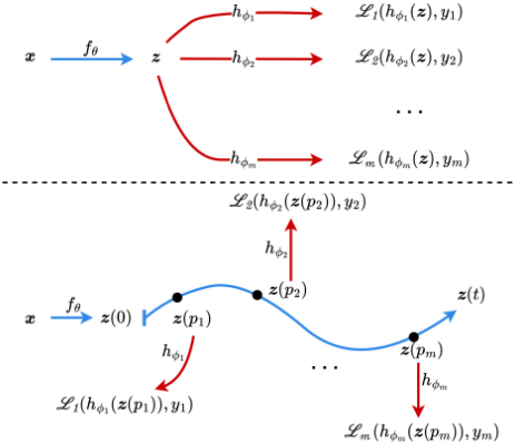
Mathematically, the objective function of the NORMAL model is formulated as
where Θ denotes all the network parameters, including φ, θ, and {ϕi}mi=1 , and Qφ(·, pi) denotes the output of the timeaware neural ODE block at task position pi. Thus, in terms of notations of NODE as introduced in the previous section, we have Qφ(fθ(xi), pi) = z(pi), where z(0) = fθ(xi).
3.2 Time-aware Neural ODE Block
In the time-aware neural ODE block, fθ(xji ) extracted by the shared feature extractor is considered as the state at initial time/position 0 in the dynamic flow, and if pi is known, then task-specific feature transformations could be learned. However, {pi} are usually unknown, and we aim to learn them.
Though first-order NODEs easily model dynamic flow, due to their instability, using them to implement Qφ often leads to poor performance. Therefore, some second-order NODE (e.g., HBNODE) is used to build this block. Specifically,
Algorithm 1 The NORMAL model.
Input: training data and learning rates µ, η Output: Task-shared parameters θ, φ, task-specific parameters {ϕi}, {pi}
- 1: for k = 1 to K do
- 2: Compute and save outputs of the time-aware neural ODE block for each task: z(pi) and q(pi);
- 3: Compute total loss L according to Eq. (6);
- 4: Compute the gradient dpi with respect to pi according to Eq. (7);
- 5: Compute the gradient ∇ΘL with respect to {θ, {ϕt}, φ};
- 6: Update Θ as Θ := Θ-µ∇ΘL;
- 7: Update pi as pi := pi - ηdpi ;
- 8: end for
based on Eq. (5), by using fθ(xji ) as the initial value z(0) of z(t) for task i, we have
where dq(l) dl = -γq(l) + g(z(l), l) + ξz(l) and a mapping function u(z) : Rn → Rn maps fθ(xji ) to the initial velocity q(0). The initial velocity mapping u(z; φv) and the ODE function g(z, t; φo) are parameterized by φv and φo, respectively. Thus, the time-aware neural ODE block Qφ is formulated as
where γ > 0 is treated a learnable parameter and ξ is treated as a hyperparameter to be tuned. To guarantee the positiveness of γ, we reparameterize it as γ = sigmoid(ω), where ω is a learnable parameter. For simplicity, we denote these parameters by φ = {φv, φo, ω}.
By using the block presented above, we can now calculate z(t) for any given initial value z(0) = fθ(xji ) and pi. Existing studies on NODEs assume that pi is available before training. In the proposed NORMAL method, if a common pi is used for all the tasks, the NODE could be absorbed into fθ(·) and different tasks could have identical feature representations, which degenerates to the HPS architecture. If different tasks use different fixed pi, setting them is too inefficient and does not have good performance according to our empirical observations. Therefore, in the NORMAL method, to achieve high expressive power in learned feature representations and low manual costs, we learn {pi} for all the tasks, which will be detailed in the next section.
3.3 Optimization
To learn parameters in the time-aware neural ODE block, we apply the adjoint sensitivity method, which can significantly reduce the memory cost during calculating the gradient. However, we cannot use auto differentiation to update {pi} since current mainstream frameworks (e.g., Tensorflow and Pytorch) do not support automatically computing the gradient for task positions {pi} in NODEs, and we need to manually compute the gradient with respect to {pi}. Specifically, for task i, the average loss Li is defined as
where z(pi) = Qφ(fθ(xji ), pi).
Based on the chain rule, we compute the gradient with respect to pi as
In Eq. (7), q(pi) denotes the output of the momentum function at time pi, which can be saved in the forward propagation process. Thus, we need to calculate the gradient of the loss Li with respect to the output of the time-aware neural ODE block at time pi. This does not require us to backpropagate the entire model, so it is not computationally expensive. Therefore, we can use dpi to update pi as pi := pi - ηdpi , where η represents the step size.
The gradients of other model parameters in the NORMAL method can be computed by auto differentiation and stochastic gradient descent methods can be used to update them. In the NORMAL method, we can update all the learnable parameters jointly or alternatively. Algorithm 1 summarizes the training algorithm for the NORMAL method.
4 RelatedWork
Multi-Task Learning. Built on the HPS architecture, there are several loss weighting and gradient manipulation methods for MTL. For example, GradNorm [Chen et al., 2018c] learns loss weights to balance the norms of the scaled gradients for different tasks. PCGrad [Yu et al., 2020] avoids the gradient conflicting between each pair of tasks by projecting the gradient of one task onto the normal plane of that of the other task. IMTL [Liu et al., 2021b] finds a descent direction that has equal projections on the gradient of each task. CAGrad [Liu et al., 2021a] minimizes the maximum of the decreasing of task losses while enforcing the update direction to be close to the average gradient among tasks. Nash-MTL [Navon et al., 2022] considers MTL as a bargaining game and finds a Nash bargaining solution. The proposed NORMAL method studies MTL from a new perspective of dynamic flow, which is different from previous works in MTL.
Neural Ordinary Differential Equation. NODEs [Chen et al., 2018b] can learn from irregularly sampled data and are particularly suitable for learning complex dynamical systems. NODE-based methods have shown promising performance on a number of tasks including building normalizing flows [Finlay et al., 2020], modeling continuous time data [Yildiz et al., 2019], and generative models [Grathwohl et al., 2019]. However, training NODEs on large datasets is not an easy task and often leads to poor performance. This is because the training process of NODE is very slow [Xia et al., 2021], and NODE often fails to learn long-term dependencies in sequential data [Lechner and Hasani, 2020]. The HBNODE [Xia et al., 2021] is based on second-order ODEs with a damping term, which can significantly accelerate the training process and provide a stable result.
5 Experiments
In this section, we empirically evaluate the proposed NORMAL method on four benchmark datasets, including Office31 [Saenko et al., 2010], Office-Home [Venkateswara et al., 2017], NYUv2 [Silberman et al., 2012], and CelebA [Liu et al., 2015]. All experiments are performed on a single NVIDIA GeForce RTX 3090 GPU.
Baselines. Here, we compare the proposed method with state-of-the-art MTL methods, including EW that adopts an equal weight on training losses of different tasks, UW [Kendall et al., 2018], GradNorm [Chen et al., 2018c], MGDA [Sener and Koltun, 2018], PCGrad [Yu et al., 2020], IMTL [Liu et al., 2021b], CAGrad [Liu et al., 2021a], and Nash-MTL [Navon et al., 2022].
Evaluation metric. For the Office-31, Office-Home, and CelebA datasets where all the tasks are classification tasks, we report the classification accuracy on each task and/or the average classification accuracy over tasks. For the NYUv2 dataset which has three tasks: 13-class semantic segmentation, depth estimation, and surface normal prediction, by following [Maninis et al., 2019], we use the average of the relative improvement of each task over the EW method as the evaluation metric, which is formulated as
where m denotes the number of tasks, Ni denotes the number of metrics for task i, M b i,j denotes the performance of an MTL method b for the jth metric in task i, M EW i,j is defined in the same way for the EW method, and si,j is set to 1 if a lower value indicates better performance for the jth metric in task i and otherwise 0.
5.1 Results on Office-31 and Office-Home Datasets
Datasets. The Office-31 dataset [Saenko et al., 2010] includes images from three different sources: images downloaded from www.amazon.com (Amazon), images from digital SLR cameras (Dslr), and images from webcams (Webcam). It contains 31 categories for each source and a total of 4652 labeled images. The Office-Home dataset [Venkateswara et al., 2017] includes images from four sources: artistic images (Ar), clip art (Cl), product images (Pr), and real-world images (Rw). It contains 65 categories for each source and a total of 15,500 labeled images. Under the multi-task learning setting, we treat each source as a separate task, so these two datasets can be used as a multi-task classification problem.
| Method | Office-31 | Office-Home | |||||||
|---|---|---|---|---|---|---|---|---|---|
| A | D | W | Avg | Ar | Cl | Pr | Rw | Avg | |
| EW | 84.67 | 98.09 | 98.70 | 93.82 | 64.77 | 79.05 | 90.11 | 80.44 | 78.59 |
| UW | 84.62 | 97.81 | 98.89 | 93.77 | 66.03 | 79.09 | 89.69 | 79.78 | 78.65 |
| GradNorm | 84.22 | 98.09 | 98.89 | 93.73 | 64.84 | 78.73 | 89.86 | 80.58 | 78.50 |
| MGDA | 78.69 | 98.09 | 98.70 | 91.83 | 65.40 | 75.05 | 89.76 | 79.96 | 77.54 |
| PCGrad | 84.67 | 97.81 | 98.70 | 93.73 | 65.27 | 78.37 | 90.08 | 79.89 | 78.40 |
| IMTL | 83.02 | 98.09 | 98.89 | 93.33 | 65.27 | 77.72 | 89.90 | 80.54 | 78.36 |
| CAGrad | 84.33 | 97.81 | 99.07 | 93.74 | 64.90 | 78.48 | 90.47 | 80.18 | 78.50 |
| Nash-MTL | 83.82 | 98.91 | 99.07 | 93.93 | 66.79 | 78.66 | 90.29 | 79.82 | 78.89 |
| NORMAL | 86.32 | 99.18 | 98.88 | 94.80 | 69.26 | 80.39 | 90.47 | 80.22 | 80.08 |
| Segmentation | Depth | Surface Normal | ||||||||
|---|---|---|---|---|---|---|---|---|---|---|
| Method | mIoU↑ | Pix Acc ↑ | Abs Err ↓ | Rel Err↓ | Angle Distance | Within t◦ | ∆ ↑ | |||
| Mean ↓ | Median ↓ | 11.25 ↑ | 22.5 ↑ | 30 ↑ | ||||||
| EW | 0.4875 | 0.7183 | 0.4179 | 0.1734 | 25.42 | 18.84 | 0.3243 | 0.5729 | 0.6845 | 0% |
| UW | 0.4866 | 0.7165 | 0.4085 | 0.1711 | 25.42 | 18.77 | 0.3212 | 0.5703 | 0.6829 | 0.45% |
| GradNorm | 0.4789 | 0.7106 | 0.4134 | 0.1686 | 25.40 | 18.61 | 0.3237 | 0.5733 | 0.6848 | 0.26% |
| MGDA | 0.4138 | 0.6631 | 0.4416 | 0.1825 | 24.33 | 17.48 | 0.3423 | 0.5975 | 0.7065 | -3.97% |
| PCGrad | 0.4835 | 0.7155 | 0.4124 | 0.1718 | 25.40 | 18.66 | 0.3230 | 0.5726 | 0.6844 | 0.21% |
| IMTL | 0.4769 | 0.7112 | 0.4141 | 0.1711 | 24.76 | 17.90 | 0.3355 | 0.5881 | 0.6978 | 0.89% |
| CAGrad | 0.4777 | 0.7113 | 0.4128 | 0.1676 | 24.80 | 17.92 | 0.3356 | 0.5874 | 0.6973 | 1.29% |
| Nash-MTL | 0.4764 | 0.7103 | 0.4155 | 0.1704 | 24.64 | 17.71 | 0.3409 | 0.5911 | 0.6999 | 1.12% |
| NORMAL | 0.4857 | 0.7184 | 0.4113 | 0.1691 | 24.98 | 18.34 | 0.3352 | 0.5827 | 0.6923 | 1.33% |
Implementation Details. On both datasets, we use a ResNet-18 network pre-trained on the ImageNet dataset as fθ, the Euler's method as the ODE solver, and a task-specific fully connected layer as the corresponding head for each task.
Implementation Details of Time-aware Neural ODE Blocks. The architectures of the initial velocity u(z; φv) and ODE function g(z, t; φo) are constructed as follows.
- Initial Velocity: →FC→LeakyReLU→FC→
- ODE Function: →FC→LeakyReLU→FC→
All the fully connected (FC) layers of both functions have a dimension of 512 for inputs and outputs.
Results. The results on the Office-31 and Office-Home datasets are shown in Table 1. We can see that on both datasets, the NORMAL method outperforms state-of-the-art baseline methods in terms of average classification accuracy. Compared with the unbalanced performance of several baseline methods on different tasks, the NORMAL method achieves a boost on almost all tasks over the EWmethod. For example, on the Office-31 dataset, the MGDA method performs well on the D and W tasks but performs very poorly on the A, which does not occur in the NORMAL method. This result demonstrates the advantage of the NORMAL method in that it can learn better feature representations for each task by learning task-specific feature transformations over dynamic flow. Moreover, compared with baselines, the proposed NORMAL method achieves the best result in some tasks, such as the best classification accuracy of 86.32% in task A for the Office-31 dataset and 69.26% classification accuracy in task Ar for the Office-Home dataset.
5.2 Results on the NYUv2 Dataset
Dataset. The NYUv2 dataset [Silberman et al., 2012] consists of video sequences of various indoor scenes recorded by RGB and Depth cameras in Microsoft Kinect. It contains 1,449 images with ground truth, where 795 images are for training and 654 images are for validation. This dataset has three tasks: 13-class semantic segmentation, depth estimation, and surface normal prediction.
Implementation Details. On the NYUv2 dataset, we use the DeepLabV3+ architecture [Chen et al., 2018a] with HBNODE. Specifically, we use pre-trained Resnet-18 with dilated convolutions [Yu et al., 2017] as the feature extractor shared by all tasks, the Euler's method as the ODE solver, and the Atrous Spatial Pyramid Pooling (ASPP) [Chen et al., 2018a] as the task-specific header for each task.
Implementation Details of Time-aware Neural ODE Blocks. The architectures of the initial velocity u(z; φv)
and ODE function g(z, t; φo) are constructed as follows.
- Initial Velocity: →Conv→LeakyReLU→Conv→
- ODE Function: →Conv→LeakyReLU→Conv→
The numbers of the input channel and output channel of the convolution layers of both functions are set to 512, the size of the kernel is 1, the stride size is 1, and the padding is 0.
Results. The results on the NYUv2 dataset are shown in Table 2. Overall, the proposed NORMAL method achieves good performance when compared with the state-of-the-art baseline methods. The MGDA method obtains the best results on all metrics of the surface normal prediction task, but performs poorly in the other two tasks, thus its overall performance is not so good. In contrast, The NORMAL method achieves relatively balanced performance on all the tasks, and hence its overall performance in terms of ∆ exceeds all other methods. This illustrates the ability of the NORMAL method to effectively improve performance on all the tasks by finding task positions.
5.3 Results on CelebADataset
Dataset. The CelebA dataset [Liu et al., 2015] includes a total of 202,599 face images and 40 face attribute annotations. In the multi-task learning setup, each face attribute is treated as a task. Thus, there are 40 classification tasks in this dataset.
Implementation Details. On the CelebA dataset, we use Resnet-18 with an average-pooling as the task-shared feature extractor fθ, the Euler's method as our ODE solver, and a fully connected layer as the task-specific head for each task.
Implementation Details of Time-aware Neural ODE Blocks. The architectures of the initial velocity u(z; φv) and ODE function g(z, t; φo) are constructed as follows.
- Initial Velocity: →FC→LeakyReLU→FC→
- ODE Function: →FC→LeakyReLU→FC→
All fully connected layers of both functions have a dimension of 2048 for both inputs and outputs.
Results. According to the results shown in Table 3, we can see that the NORMAL method achieves the best average classification accuracy performance on the CelebA dataset, which again demonstrates the effectiveness of the NORMAL method.
| Method | Avg |
|---|---|
| EW | 90.78 |
| UW | 90.82 |
| GradNorm | 90.69 |
| MGDA | 90.40 |
| PCGrad | 90.93 |
| IMTL | 90.46 |
| CAGrad | 90.73 |
| Nash-MTL | 90.83 |
| NORMAL | 91.00 |
5.4 Analysis on Learned Task Positions
In this section, we analyze the learned task positions {pi} to see why the NORMAL method achieves good performance on these datasets.
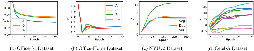
The training curves of all {pi} on the four benchmark datasets are shown in Figure 2, where due to the large number of tasks in the CelebA dataset, we randomly select a portion of the tasks for better illustration. According to Figure 2, we have two observations.
Firstly, the proposed NORMAL method does successfully learn task positions. Taking the training curves of {pi} on the NYUv2 dataset in Figure 2(c) as an example, we can see that its training trajectory is very smooth and all task positions eventually converge to their own convergent points. We can also find similar results in Figures 2(a) and 2(b). In Figure 2(d), though the training trajectory is not as smooth as the other three datasets, the proposed NORMAL method can still differentiate tasks and find their own task positions.
Secondly, {pi} learned by the NORMAL method are able to reflect task relations. For example, according to Figures 2(a) and 2(b), the task positions in these two datasets converge to a very similar value. This result is consistent with the nature of the Office-31 and the Office-Home datasets in that different tasks in each dataset are semantically similar due to the shared label space among tasks. In Figure 2(c), we find that psur learned for the surface normal prediction task is different from pseg and pdep learned for the semantic segmentation and depth estimation tasks, which indicates that the surface normal prediction task is not so related to the other two tasks, and this observation matches some previous study [Sun et al., 2021], which verifies that the learned {pi} can reflect task relations. In Figure 2(d), we can see that different tasks tend to form several groups based on learned task positions {pi}. For example, some tasks (e.g., Sideburns and Wavy Hair) have similar task positions as face attributes corresponding to those tasks are similar. Moreover, some tasks (e.g., Receding Hairline and 5 o Clock Shadow) have different task positions since face attributes corresponding to those tasks are totally different. Those results show that the learned task positions could help identify task clusters.
| Office-31 | Office-Home | ||||||||
|---|---|---|---|---|---|---|---|---|---|
| Setting | A | D | W | Avg | Ar | Cl | Pr | Rw | Avg |
| Constant and identical {pi} | 84.62 | 98.36 | 98.89 | 93.95 | 61.35 | 75.37 | 87.75 | 75.28 | 74.94 |
| Constant but different {pi} | 85.24 | 98.36 | 98.52 | 94.04 | 61.35 | 75.37 | 87.75 | 75.28 | 74.94 |
| Different form of pi: pi = eνi | 85.47 | 97.81 | 98.70 | 94.00 | 68.82 | 79.23 | 89.55 | 80.68 | 79.57 |
| Using first-order NODE | 84.79 | 98.36 | 98.89 | 94.01 | 65.27 | 77.57 | 88.98 | 76.97 | 77.45 |
| Adding task-shared layers | 83.87 | 97.81 | 98.15 | 93.28 | 58.13 | 73.28 | 85.06 | 72.43 | 72.22 |
| Adding task-specific layers | 83.87 | 97.81 | 97.59 | 93.09 | 60.34 | 74.50 | 87.25 | 74.31 | 74.10 |
| NORMAL | 86.32 | 99.18 | 98.88 | 94.80 | 69.26 | 80.39 | 90.47 | 80.22 | 80.08 |
In summary, the proposed NORMAL method could learn meaningful task positions that can reveal task relations.
5.5 Ablation Studies
In this section, we conduct ablation studies on the Office-31 and Office-Home datasets to answer several questions which are placed at the beginning of the following paragraphs.
Are the learned task positions advantageous compared with fixed task positions? We try to use a fixed parameter p shared by all tasks and use task-specific fixed parameters {pi} for different tasks. For the former setting, we use p = 1. In the latter setting, for the Office-31 dataset, we try to set task positions of the three tasks to each permutation of a set {1, 1.25, 1.5} and select the best performed one, and for the Office-Home dataset, the set to generate task positions is {1, 1.25, 1.5, 1.75}. According to the results shown in Table 4, the performance of the two settings for task positions is inferior to the learning of task positions in the proposed NORMAL method, which demonstrates the effectiveness of the learning strategy for task positions in the NORMAL method.
How do different forms of learning task positions impact the performance? Here we try positive task positions and parameterize task positions {pi} as pi = eνi . As shown in Table 4, the model learned here is inferior to that of the NORMAL model without any constraint on task positions by 0.80% and 0.51% on the Office-31 and Office-Home datasets, respectively, which shows that learning task positions without the positive requirement may be better. Based on Tables 1 and 4, this variant to learn positive task positions still performs better than baseline methods, which again verifies the effectiveness of the NORMAL method.
How do different NODE algorithms impact the performance? The NORMAL method uses a second-order ODE method but not first-order NODEs. Here we explore whether different methods in the NODE family impact the performance of the NORMAL method. We evaluate the performance of the NORMAL method using the first-order NODE [Chen et al., 2018b]. According to results shown in Tables 1 and 4, we can see that on the Office-Home dataset, the performance of the NORMAL method using the firstorder NODE method is worse than the NORMAL method and baseline methods. Some possible reasons are that first-order NODEs usually cannot be trained stably and that secondorder NODEs are more expressive. For the Office-31 dataset, the NORMAL method with the first-order NODE performs slightly worse than the NORMAL method but slightly better than the baseline methods. One possible reason is that the Office-31 dataset is easier than the Office-Home dataset. In summary, second-order NODE methods are preferred to be used in the NORMAL method.
Does the enhancement of the NORMAL method result fromthe addition of certainparameters? The time-aware neural ODE block in the NORMAL method introduces a small number of parameters, which are almost negligible compared to other model parameters. We aim to investigate whether such an increasing number of parameters brings performance gain. Therefore, we experiment to add task-shared layers in fθ and task-specific layers in {hϕi }, respectively, to match with the number of parameters in NORMAL method, and show results in Table 4. According to the results, we can see that the introduction of additional layers does not bring a performance improvement, and even lead to performance degradation. One possible reason could be the overfitting issue. Through this experiment, we can see that the performance of the NORMAL method is attributed from the entire model design but not the introduction of more parameters.
6 Conclusion
In this work, we propose the NORMAL algorithm to model multiple learning tasks from the perspective of dynamic flow. By learning the task positions in the NODE, the NORMAL method can model the task relations in terms of the relative task positions. Experiments on benchmark datasets demonstrate the effectiveness of the proposed NORMAL method.
Acknowledgments
This work is supported by NSFC key grant under grant no. 62136005, NSFC general grant under grant no. 62076118, and Shenzhen fundamental research program JCYJ20210324105000003.
Contribution Statement
Feiyang Ye and Xuehao Wang contributed equally to this work.
@inproceedings{ijcai2023p500,
  title     = {Multi-Task Learning via Time-Aware Neural ODE},
  author    = {Ye, Feiyang and Wang, Xuehao and Zhang, Yu and Tsang, Ivor W.},
  booktitle = {Proceedings of the Thirty-Second International Joint Conference on
               Artificial Intelligence, {IJCAI-23}},
  publisher = {International Joint Conferences on Artificial Intelligence Organization},
  editor    = {Edith Elkind},
  pages     = {4495--4503},
  year      = {2023},
  month     = {8},
  note      = {Main Track},
  doi       = {10.24963/ijcai.2023/500},
  url       = {https://doi.org/10.24963/ijcai.2023/500},
}
TY - CPAPER TI - Multi-Task Learning via Time-Aware Neural ODE AU - Ye, Feiyang AU - Wang, Xuehao AU - Zhang, Yu AU - Tsang, Ivor W. T2 - Proceedings of the Thirty-Second International Joint Conference on Artificial Intelligence, IJCAI-23 PB - International Joint Conferences on Artificial Intelligence Organization PY - 2023 SP - 4495 EP - 4503 DO - 10.24963/ijcai.2023/500 UR - https://doi.org/10.24963/ijcai.2023/500 ER -Copied
Machine-readable versions of this paper, for tools and AI agents:





