
Learning to Binarize Continuous Features for Neuro-Rule Networks
Proceedings of the Thirty-Second International Joint Conference on Artificial Intelligence. Main Track. Pages 4584-4592.
https://doi.org/10.24963/ijcai.2023/510
Keywords
- Machine Learning: ML: Neuro-symbolic methods
Abstract
Neuro-Rule Networks (NRNs) emerge as a promising neuro-symbolic method, enjoyed by the ability to equate fully-connected neural networks with logic rules. To support learning logic rules consisting of boolean variables, converting input features into binary representations is required. Different from discrete features that could be directly transformed by one-hot encodings, continuous features need to be binarized based on some numerical intervals. Existing studies usually select the bound values of intervals based on empirical strategies (e.g., equal-width interval). However, it is not optimal since the bounds are fixed and cannot be optimized to accommodate the ultimate training target. In this paper, we propose AutoInt, an approach that automatically binarizes continuous features and enables the intervals to be optimized with NRNs in an end-to-end fashion. Specifically, AutoInt automatically selects an interval for a given continuous feature in a soft manner to enable a differentiable learning procedure of interval-related parameters. Moreover, it introduces an additional soft K-means clustering loss to make the interval centres approach the original feature value distribution, thus reducing the risk of overfitting intervals. We conduct comprehensive experiments on public datasets and demonstrate the effectiveness of AutoInt in boosting the performance of NRNs.
- [Alexander and Mozer, 1994] Jay A. Alexander and Michael Mozer. Template-based algorithms for connectionist rule extraction. In NeurIPS, pages 609-616, 1994.
- [Bengio et al., 2013] Yoshua Bengio, Nicholas Léonard, and Aaron Courville. Estimating or propagating gradients through stochastic neurons for conditional computation. arXiv preprint arXiv:1308.3432, 2013.
- [Bezdek, 2013] James C Bezdek. Pattern recognition with fuzzy objective function algorithms. Springer Science & Business Media, 2013.
- [Castelvecchi, 2016] Davide Castelvecchi. Can we open the black box of ai? Nature News, 538(7623):20, 2016.
- [Cheng et al., 2022] Kewei Cheng, Jiahao Liu, Wei Wang, and Yizhou Sun. Rlogic: Recursive logical rule learning from knowledge graphs. In KDD, pages 179-189, 2022.
- [Dehaspe and Toivonen, 1999] Luc Dehaspe and Hannu Toivonen. Discovery of frequent DATALOG patterns. Data Min. Knowl. Discov., 3(1):7-36, 1999.
- [Dong et al., 2019] Honghua Dong, Jiayuan Mao, Tian Lin, Chong Wang, Lihong Li, and Denny Zhou. Neural logic machines. In ICLR, 2019.
- [Dougherty et al., 1995] James Dougherty, Ron Kohavi, and Mehran Sahami. Supervised and unsupervised discretiza- tion of continuous features. In ICML, pages 194-202, 1995.
- [Fard et al., 2020] Maziar Moradi Fard, Thibaut Thonet, and Éric Gaussier. Deep k-means: Jointly clustering with k- means and learning representations. Pattern Recognit. Lett., 138:185-192, 2020.
- [Garcez et al., 2022] Artur d'Avila Garcez, Sebastian Bader, Howard Bowman, Luis C Lamb, Leo de Penning, BV Il- luminoo, Hoifung Poon, and COPPE Gerson Zaverucha. Neural-symbolic learning and reasoning: A survey and in- terpretation. Neuro-Symbolic Artificial Intelligence: The State of the Art, 342:1, 2022.
- [Glanois et al., 2022] Claire Glanois, Zhaohui Jiang, Xuen- ing Feng, Paul Weng, Matthieu Zimmer, Dong Li, Wulong Liu, and Jianye Hao. Neuro-symbolic hierarchical rule in- duction. In ICML, pages 7583-7615, 2022.
- [Hu et al., 2016] Zhiting Hu, Xuezhe Ma, Zhengzhong Liu, Eduard H. Hovy, and Eric P. Xing. Harnessing deep neural networks with logic rules. In ACL, 2016.
- [Jin et al., 2022] Yang Jin, Linchao Zhu, and Yadong Mu. Complex video action reasoning via learnable markov logic network. In CVPR, pages 3232-3241, 2022.
- [Liu and Setiono, 1997] Huan Liu and Rudy Setiono. Fea- ture selection via discretization. IEEE Trans. Knowl. Data Eng., 9(4):642-645, 1997.
- [Manhaeve et al., 2018] Robin Manhaeve, Sebastijan Du- mancic, Angelika Kimmig, Thomas Demeester, and Luc De Raedt. Deepproblog: Neural probabilistic logic programming. In NeurIPS, pages 3753-3763, 2018.
- [Marra and Kuzelka, 2021] Giuseppe Marra and Ondrej Kuzelka. Neural markov logic networks. In UAI, pages 908-917, 2021.
- [Marra et al., 2020] Giuseppe Marra, Sebastijan Dumancic, Robin Manhaeve, and Luc De Raedt. From statistical re- lational to neural symbolic artificial intelligence: a survey. In IJCAI, pages 4943-4950, 2020.
- [Meilicke et al., 2019] Christian Meilicke, Melisachew Wudage Chekol, Daniel Ruffinelli, and Heiner Stuckenschmidt. Anytime bottom-up rule learn- ing for knowledge graph completion. In IJCAI, pages 3137-3143, 2019. IJCAI
- [Qiao et al., 2021] Litao Qiao, Weijia Wang, and Bill Lin. Learning accurate and interpretable decision rule sets from neural networks. In AAAI, pages 4303-4311, 2021.
- [Qu and Tang, 2019] Meng Qu and Jian Tang. Probabilistic logic neural networks for reasoning. In NeurIPS, pages 7710-7720, 2019.
- [Qu et al., 2021] Meng Qu, Junkun Chen, Louis-Pascal A. C. Xhonneux, Yoshua Bengio, and Jian Tang. Rnn- logic: Learning logic rules for reasoning on knowledge graphs. In ICLR, 2021.
- [Quinlan, 2014] J Ross Quinlan. C4. 5: programs for ma- chine learning. Elsevier, 2014.
- [Rudin, 2019] Cynthia Rudin. Stop explaining black box machine learning models for high stakes decisions and use interpretable models instead. Nature Machine Intelligence, 1(5):206-215, 2019.
- [Sarker et al., 2021] Md Kamruzzaman Sarker, Lu Zhou, Aaron Eberhart, and Pascal Hitzler. Neuro-symbolic artificial intelligence: Current trends. arXiv preprint arXiv:2105.05330, 2021.
- [Sharmin et al., 2019] Sadia Sharmin, Mohammad Shoyaib, Amin Ahsan Ali, Muhammad Asif Hossain Khan, and Oksam Chae. Simultaneous feature selection and dis- cretization based on mutual information. Pattern Recog- nit., 91:162-174, 2019.
- [Wang et al., 2020] Zhuo Wang, Wei Zhang, Ning Liu, and Jianyong Wang. Transparent classification with multilayer logical perceptrons and random binarization. In AAAI, pages 6331-6339, 2020.
- [Wang et al., 2021] Zhuo Wang, Wei Zhang, Ning Liu, and Jianyong Wang. Scalable rule-based representation learn- ing for interpretable classification. In NeurIPS, 2021.
- [Xie et al., 2019] Yaqi Xie, Ziwei Xu, Kuldeep S. Meel, Mo- han S. Kankanhalli, and Harold Soh. Embedding symbolic knowledge into deep networks. In NeurIPS, pages 4235- 4245, 2019.
- [Yadav et al., 2021] Rohan Kumar Yadav, Lei Jiao, Ole- Christoffer Granmo, and Morten Goodwin. Human-level interpretable learning for aspect-based sentiment analysis. In AAAI, pages 14203-14212, 2021.
- [Yang et al., 2017] Fan Yang, Zhilin Yang, and William W. Cohen. Differentiable learning of logical rules for knowl- edge base reasoning. In NeurIPS, pages 2319-2328, 2017.
- [Yang et al., 2022] Zhun Yang, Joohyung Lee, and Chiyoun Park. Injecting logical constraints into neural networks via straight-through estimators. In ICML, pages 25096- 25122, 2022.
- [Zhang et al., 2022a] Wei Zhang, Junbing Yan, Zhuo Wang, and Jianyong Wang. Neuro-symbolic interpretable collab- orative filtering for attribute-based recommendation. In WWW, pages 3229-3238, 2022.
- [Zhang et al., 2022b] Yao Zhang, Yun Xiong, Yiheng Sun, Caihua Shan, Tian Lu, Hui Song, and Yangyong Zhu. Rudi: Explaining behavior sequence models by automatic statistics generation and rule distillation. In CIKM, pages 2651-2660, 2022.
References were extracted automatically from the PDF and may contain errors.
Full text extracted automatically from the PDF; figures, tables and equations may differ. The PDF is the version of record.
1 Introduction
In the last decade, deep neural networks have become the representative achievement of Artificial Intelligence (AI) and gained overwhelming success in diverse areas. However, the intrinsic black-box nature [Castelvecchi, 2016] of deep neural networks hinders their applications in high-stake domains, such as finance, education, and healthcare [Rudin, 2019]. In contrast to deep neural networks, the symbolic approaches in the first generation of AI possess high interpretability and a strong logical reasoning ability, yet they usually suffer from worse performance. To combine the merits of deep neural networks and symbolic computation, the research community has started to resort to neuro-symbolic AI [Marra et al., 2020;
| Marital | Height | |
|---|---|---|
| 1 | married | 1.73 |
| 2 | single | 1.65 |
| 3 | married | 1.58 |
| 4 | divorced | 1.85 |
| 5 | single | 1.79 |
| 6 | married | 2.08 |
Sarker et al., 2021; Garcez et al., 2022]. It is believed to be a vital technical direction towards the next generation of AI.
The past several years have witnessed gratifying progress in some research subfields of neuro-symbolic AI, like neural logic programming for proving [Manhaeve et al., 2018] and neural Markov logic network for incorporating rules [Qu and Tang, 2019; Marra and Kuzelka, 2021]. Different from them, the recently proposed Neuro-Rule Networks (NRNs) [Wang et al., 2020; Qiao et al., 2021; Wang et al., 2021] are a novel type of neuro-symbolic method. Their impressive character is to equate fully-connected neural networks with logic rules, and thus neural networks and logic rules have the same reasoning process. This is remarkable progress in logic rule learning through neural networks and is in contrast to the approaches requiring knowledge graphs [Meilicke et al., 2019; Cheng et al., 2022] or pre-defined meta-rules [Glanois et al., 2022]. Due to the advantages in both accuracy and interpretability, NRNs have been successfully applied to domains such as explainable product recommendation [Zhang et al., 2022a], financial fraud detection [Zhang et al., 2022b], etc.
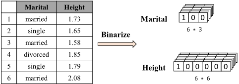
A logic rule uses operations such as conjunction (AND, ∧) and disjunction (OR, ∨) to combine some Boolean variables to generate inference results. A Boolean variable takes value one (True) if a given feature satisfies the corresponding condition, and otherwise, it takes value zero (False). NRNs require the input to take binary values, facilitating logic rule learning. For categorical features, it is straightforward to utilize one-hot encoding to transform them into binary vectors, the size of which is equal to the number of categories. However, using the same strategy for binarizing continuous features is infeasible. As shown in Figure 1, after transformation by onehot encoding, the size of the binary vector for the continuous feature (i.e., Height) is much larger than that for the categorical feature (i.e., Marital). In theory, the number of values a continuous feature can take is infinite. As such, this will lead to high-dimensional and very sparse vectors, which inevitably increases the difficulty of optimization To reduce the dimension of binarized continuous feature vectors, some studies [Wang et al., 2020; Qiao et al., 2021; Wang et al., 2021] resort to interval-based binarization. In this way, the dimension equals the number of intervals. However, these studies employ empirical strategies to determine the bound values of intervals, such as random bound sampling and equal-width interval, and fix them during the training process. This loses the chance of optimizing the interval bounds with the overall NRNs, which might be suboptimal for ultimate task performance. Although regarding the bound values as parameters to be automatically learned is promising and intuitive, there are two main technical challenges to be resolved: (1) The procedure of interval-based binarization is not differentiable w.r.t. bound parameters and thus commonly-adopted optimization methods for neural networks like gradient back-propagation could not be directly applied. (2) The learned intervals should match the original feature value distribution to some extent, which is also beneficial for reducing the risk of overfitting the intervals.
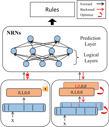
In this paper, we propose a new approach, named AutoInt, to automatically optimize intervals with NRNs in an end-toend fashion. As shown in Figure 2, compared to fixing intervals during training, AutoInt iteratively updates the intervals to make them adapt to the overall model during training. Specifically, for the first challenge, AutoInt calculates the distances between a feature value and interval centres, and uses the distances to represent the probabilities that the feature value belongs to different intervals. The soft probability vector is further leveraged to derive an approximate binary input vector. Benefiting from this, the learning procedure of interval-related parameters is differentiable. For the second challenge, AutoInt exploits K-means to cluster feature values and takes the cluster centers equivalent to interval centres. An additional soft K-means clustering loss is introduced to optimize interval centres jointly with the main target loss to approach the original feature value distribution.
To sum up, the contributions of this paper are as follows:
- A differentiable binarization methodology is proposed, enabling the automatic optimization of intervals with NRNs in an end-to-end fashion.
- A soft K-means clustering loss is used in conjunction with an ultimate task loss to make the learned intervals approach the original feature value distribution.
- Comprehensive experiments on several public datasets with continuous features demonstrate the effectiveness of AutoInt over conventional feature binarization approaches. The source code of AutoInt is available at https://github. com/yxliu99/AutoInt.
2 Preliminaries
2.1 Neuro-Rule Networks
Neuro-rule networks are actually a type of fully-connected neural network but with some special designs. Firstly, logical activation functions are devised to replace standard action functions (e.g., ReLU). They are the key factor to imitate conjunction and disjunction operations for forming logic rules. One of the main differences between different NRNs also lies in the instantiations of logical activation functions. Secondly, all the parameters of NRNs except for the last layer are constrained in the range of [0, 1] and the input is also required to have binary values. This is because logic rules consist of Boolean variables that take a value of zero or one.
From the overall perspective, NRNs are composed of a binarization layer, several logical layers, and a prediction (inference) layer. The binarization layer is responsible for converting all categorical and continuous features to binary values. The logical layer is the core part of NRNs. It involves the aforementioned logical activation functions and uses the constrained weights to connect different layers. The prediction layer makes the final estimation for a given instance. In some NRNs, this layer could calculate the rule importance by assigning rules with different weights.
2.2 ProblemFormulation
Let D = {(X1, y1), . . . , (XN, yN)} denote the training data set, where N is the size. Xi denotes the features of the i-th instance in the set and yi is the corresponding ground-truth class. Assume Xi involves both categorical features (X′ i ) and continuous features (X′′ i ), then Xi = {X′ i , X′′ i }. For the categorical features, it is straightforward to use one-hot encoding to convert them to binary vectors (e.g., x′i,1 for the first categorical feature). Then the feature value vector of Xi is formulated as follows:
where M ′ and M ′′ represent the number of categorical and continuous features, respectively. x′′ i,1 is the value of the 1st continuous feature. Based on the notations, we define the studied problem in the following.
Problem (Continuous Feature Binarization for Neuro-Rule Networks). Given a neuro-rule network NRN and a feature value vector ¯xi, the goal of this problem is to pursue a continuous feature binarization function f that is compatible with the network for better inferring the label ˆ yi, defined as
For brevity, we omit the subscripts and superscripts, and use x as the value of a given continuous feature, which is later used for illustrating the proposed approach.
3 Methodology
In this section, we first give an overview of the proposed AutoInt. Then we go into the details of two critical modules of AutoInt. Finally, we introduce how to optimize AutoInt, along with the neuro-rule network.
3.1 Overview
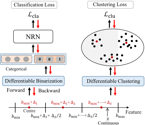
As shown in Figure 3, AutoInt mainly contains two modules. The differential binarization module serves NRNs by converting input continuous features to binary vectors, which are further concatenated with categorical features and fed into NRNs. The differential clustering module is responsible for clustering feature values and associating cluster centers with interval centres. Moreover, both the classification loss and clustering loss are leveraged to jointly optimize intervals.
3.2 Interval-based Differentiable Feature Binarization
Interval Bound Representation
To binarize continuous features, AutoInt utilizes the intervalbased discretization technique. Specifically, for a given continuous feature, let the minimal value and the maximal value that the feature can take be denoted as bmin and bmax, respectively. We specify the number of intervals for the feature to be K. Then an intuitive way to represent the intervals is [bmin, b1], (b1, b2], · · · , (bK-1, bmax], where {bk}k=K-1 k=1 are the interval bound values.
Since the main goal of AutoInt is to optimize the intervals, it is natural to regard the bound values (except for bmin and bmax) as trainable parameters. However, directly optimizing them poses a risk that the partial order relation of the bound values (i.e., b1 < b2 < · · · < bK-1) might be changed when they are iteratively updated during the training process. This will lead to invalid intervals and adversely affect the accuracy of logic rules. To tackle this, we consider an increment-based interval representation manner. Firstly, we define increments {δk}k=K-1 k=1 , wherein δk is the width of the k-th interval and should be larger than zero. Furthermore, we utilize the increments to represent intervals as follows: [bmin, bmin +δ1], (bmin +δ1, bmin +δ1 +δ2], · · · , (bmin + δ1 + · · · + δK-1, bmax].
Interval Selection
Based on the above intervals, a simple way to get the binary vector x for a given feature value x is hard selection defined as follows:
However, the above computational procedure is not differentiable w.r.t. {δk}k=K-1 k=1 , since the corresponding function is not continuous in the value range of x and the parameters only occur in the condition terms.
To enable the learning procedure of bound parameters differentiable, we resort to soft selection by calculating the probability that a feature value belongs to an interval. For continuous features, it is natural to use the distance between a feature value and the centre of an interval to derive the probability. The centre can be calculated by averaging the lower bound and upper bound of its interval. For example, the centre of the k-th interval is bmin + δ1 + · · · + δk-1 + δk/2. Nevertheless, using this type of centres to compute the distance and probability will cause inconsistency in rule construction. Suppose there are two given intervals, i.e., [1, 2] with centre 1.5 and (2, 6] with centre 4. For a feature value 2.5, its distance with the first interval is smaller than that with the second interval. Therefore the probability that the feature belongs to the first interval is larger. However, we can easily find that 2.5 is actually within the interval (2, 6].
To tackle the aforementioned problem, we propose first representing interval centres based on increments and then determining interval bounds based on the centres. As shown at the bottom part of Figure 3, AutoInt uses increments
{∆k}k=K k=1 . For the k-th interval, the corresponding centre ck is formulated as
Consequently, the lower and the upper bounds of the interval are bmin + · · · +∆k/2 and bmin + · · · +∆k +∆k+1/2, respectively. Note that the centre ck is not exactly the true centre, since it is very likely that ∆k ̸= ∆k+1. However, this way could ensure the correctness of the logic rule construction, which is a top priority for NRNs. Considering this reason, AutoInt takes the pseudo centres {ck}k=K k=1 as the interval centres throughout this paper.
Based on the obtained centres, we can calculate the probabilities of the value belonging to different intervals. The computational formula is formulated as follows:
where D denotes a distance function and squared distance is used. τ1 is a hyper-parameter to control the sharpness of the distribution. Thanks to this soft selection manner, the trainable parameters {∆k}k=K k=1 are moved from condition terms (similar as Equation 1) to the main computational graph. Based on the probability distribution p, AutoInt selects the interval that has the largest probability and obtains the binary vector b through the following function:
This function is not differentiable w.r.t. {∆k}k=K k=1 and we will show how to settle this problem in Section 3.4. Now b can be fed into an NRN for label inference.
3.3 Differentiable Clustering for Interval Centres
Besides being used for continuous feature binarization, the learned intervals should also match the original feature value distribution to some extent. This is advantageous because it could reduce the risk of overfitting and make them more robust towards the training process. To realize this, we propose to cluster the feature values occurring in a given dataset. This is motivated by the fact that clusters could reflect the characteristics of the value distribution. Moreover, cluster center points are associated with interval centres. In this way, the number of clusters is equal to the number of intervals. As a result, the clustering process could affect the optimization of intervals.
To make the objective function of clustering differentiable w.r.t. the interval-related parameters, we adopt the soft Kmeans clustering algorithm [Bezdek, 2013; Fard et al., 2020] (note that AutoInt can also use other differentiable clustering algorithms). Specifically, the probability ¯ pk that x belongs to the k-th cluster is computed in a similar fashion as Equation 3. The only difference is the introduction of another hyper-parameter τ2 with the same role. Afterwards, we define the K-means clustering loss for this feature value as follows:
| Dataset | #instances | #classes | #total features | #continuous features |
|---|---|---|---|---|
| adult | 32561 | 2 | 14 | 6 |
| bank | 45211 | 2 | 16 | 7 |
| credit | 30000 | 2 | 23 | 14 |
| redwineQ | 1599 | 6 | 11 | 11 |
| whitewineQ | 4898 | 7 | 11 | 11 |
| wine | 178 | 3 | 13 | 13 |
The above loss could be easily extended to include all the continuous features in a training set.
3.4 Optimization
Since the intervals are optimized with a neuro-rule network, we first use Lcla to represent the classification loss for the whole network. Then backward computation flow from the loss to {∆k}k=K k=1 should be generated. However, this flow is blocked by Equation 4 which is not differentiable. To open the blocked flow, we adopt the straight-through estimator (STE) [Bengio et al., 2013], an approximate method that uses the binary vector b for forward computation (inference) and the probability distribution p as an approximation for backward computation (gradient optimization). When τ1 in Equation 3 takes a large value, the distribution becomes sharp and could approximate the binary vector well. Specifically, it inserts the following computation formula between the probability distribution p and the binary vector b,
where Stop-grad denotes stopping the gradient computation. The final optimization target for AutoInt is as follows:
where λ is a hyper-parameter to control the relative influence of Lclu. Considering the constraints that ∆k (k ∈ {1, · · · ,K}) must take positive values, we use the simple trick, i.e., ∆k = max(∆k, ϵ), during the training process. ϵ is a very small positive constant (e.g., 1e-3).
All the trainable parameters introduced by AutoInt are only {∆k}k=K k=1 for each continuous feature. Suppose the number of continuous features is M ′′ . Then the total number of parameters is KM ′′ , which is usually small and not affected by the number of instances in a dataset. Therefore, AutoInt brings a very low space overhead to train NRNs. Besides, although the training time of NRNs becomes longer, the complexity of inference time is the same as the original NRNs. This is attributed to the fact that the learned intervals can be easily stored after training and all the modules of AutoInt will be removed when performing inference.
4 Experiments
4.1 Experimental Setup
In the experimental setup, we describe the datasets used for experiments, the baselines adopted for comparison, and the implementation details.
| Dataset | XGBoost | RanInt | WidInt | FreInt | KInt | EntInt | RanInt+ | WidInt+ | FreInt+ | KInt+ | EntInt+ | AutoInt |
|---|---|---|---|---|---|---|---|---|---|---|---|---|
| adult | 80.64 | 80.72 | 80.47 | 79.84 | 80.59 | 80.70 | 78.30 | 79.60 | 78.79 | 79.84 | 78.64 | 80.74 |
| bank | 74.71 | 76.32 | 75.72 | 75.89 | 76.34 | 76.48 | 74.39 | 75.35 | 75.67 | 75.91 | 75.45 | 77.59 |
| credit | 68.04 | 69.96 | 69.85 | 69.86 | 69.92 | 69.87 | 68.55 | 69.82 | 69.94 | 69.95 | 69.88 | 70.54 |
| redwineQ | 37.22 | 35.78 | 35.58 | 35.55 | 35.86 | 34.79 | 33.09 | 33.36 | 33.42 | 34.07 | 33.25 | 37.53 |
| whitewineQ | 43.78 | 39.21 | 39.48 | 39.07 | 39.53 | 38.79 | 36.61 | 37.75 | 38.34 | 38.66 | 37.24 | 40.93 |
| wine | 97.78 | 98.23 | 97.40 | 97.73 | 97.74 | 97.73 | 96.62 | 96.89 | 97.16 | 96.80 | 96.65 | 99.01 |
Datasets
We use six public datasets from the UCI dataset repository 1 . All of them satisfy to contain some continuous features for testing the effectiveness of binarization methods. Table 1 summarizes the statistics of the 6 datasets. The number of continuous features ranges from 6 to 14 in the experiments, occupying large ratios in total. Considering that all these datasets are used for classification and the instance counts of different classes are imbalanced, we adopt the F1 score (Macro) as the evaluation metric.
Baselines
We compare the following continuous feature binarization methods with the proposed AutoInt:
- Random interval sampling (RanInt) is adopted by RRL [Wang et al., 2021], which determines interval bounds through random sampling from a uniform distribution.
- Equal-width interval (WidInt) is leveraged by Qiao et al. [2021]. It partitions the value range of a feature into K intervals with an equal width.
- Equal-frequency interval (FreInt), summarized in [Dougherty et al., 1995], divides a feature into K intervals where each interval contains nearly the same number of feature values.
- K-means clustering-based interval (KInt), also summarized in [Dougherty et al., 1995], utilizes K-means to cluster feature values into K clusters. Interval bounds are straightforwardly obtained based on the clusters.
- Recursive minimal entropy partitioning (EntInt) [Wang et al., 2020] is an entropy-based method that recursively partitions feature values according to the class information entropy of each candidate partition.
Considering RRL [Wang et al., 2021] is the SOTA neurorule network, we train it with different feature binarization methods in the experiments. It is noteworthy that RRL uses another interval type where different intervals have overlaps (e.g, [bmin, b2], (bmin, b3], [bmin, b4] where bmin < b2 < b3 < b4). For a comprehensive study, we test binarization methods using both overlapping and non-overlapping intervals. To distinguish one from another, we use RanInt to represent using overlapping intervals and RanInt+ to denote using non-overlapping intervals, and the same is true for other baseline methods.
1 https://archive.ics.uci.edu/ml/datasets.php
Implementation Details
To have a reliable performance evaluation, we adopt 5fold cross-validation and report the average performance, the same as [Wang et al., 2021]. When there are hyperparameters needing to be tuned, we use 80% of the training set for optimization and the left for validation. For the neuro-rule network RRL and XGBoost (XGBoost directly uses the continuous features as input), we also follow [Wang et al., 2021] to set their hyper-parameters. For the proposed AutoInt, both the temperature τ1 and τ2 are selected in {500, 1000, 2000}, K is searched in {5, 10, 15, 20, 30, 50}, and λ is tuned in {0.005, 0.01, 0.05, 0.1, 0.2, 0.5}. The intervals are initialized by FreInt, if not otherwise stated. Besides, all the continuous feature values are pre-processed through standard normalization.
4.2 Overall Performance
The overall performance of different binarization methods on six datasets is presented in Table 2. XGBoost is used as a reference because it is generally acknowledged as a wellperformed model in different classification tasks. Based on the results, we have the following observations:
- The results of the baseline methods using overlapping intervals are better than the baseline methods using nonoverlapping intervals in most cases. The main reason might be that the sparsity of binary vectors obtained through overlapping and non-overlapping intervals are apparently different. For the former one, the obtained binary vector is very likely to have multiple non-zero entries. By contrast, non-overlapping intervals definitely lead to one-hot vectors, which are much sparser. As a result, using non-overlapping intervals for binarization might increase the training difficulty of NRNs a little bit.
- By comparing the performance of the baseline methods using the same type of intervals, it can be concluded that each method has its own merits. One counterintuitive aspect is that RanInt is competitive among the baselines. This could be explained by the following reason. RanInt might randomly generate some good intervals than other unlearnable interval schemes for RRL and the effect of the generated inferior intervals is alleviated for overlapping intervals.
- AutoInt behaves much better than the baseline binarization methods that also use non-overlapping intervals. This demonstrates that through optimizing intervals with NRNs, AutoInt obtains intervals compatible with the final classification ask. Moreover, AutoInt also outperforms XGBoost and the baseline methods that utilize overlapping intervals.
| Dataset | AutoInt | w/o Clu. Loss | AutoInt(Fixed) |
|---|---|---|---|
| adult bank credit redwineQ whitewineQ wine | 80.74 | 80.29 | 78.79 |
| 77.59 | 76.85 | 75.67 | |
| 70.54 | 70.04 | 69.94 | |
| 37.53 | 35.18 | 33.42 | |
| 40.93 | 38.83 | 38.34 | |
| 99.01 | 97.31 | 97.16 |
In summary, the superiority of AutoInt is validated, showing that optimizing intervals is promising.
- AutoInt is not applied to overlapping intervals. This is because AutoInt relies on measuring the distance between a feature value and interval centres. And the interval with the shortest distance (the largest probability) is selected. If the intervals are overlapped, it is not easy to use distance to select the most probable interval. Moreover, we have also tried using the sigmoid function (σ) to approximate the binarization process of using overlapping intervals. To be specific, if x > bk, we let σ(x - bk) approach value zero, and otherwise, we let it approach value one. However, this method does not exhibit performance improvements in our local experiments.
4.3 Ablation Study
An ablation study is further conducted to show the contributions of the key modules in AutoInt. We consider the following two variants: (1) "w/o Clu. Loss" denotes removing the module of differentiable clustering. (2) "AutoInt(Fixed)" represents removing both differentiable binarization and differentiable clustering, equivalent to fixing the interval bounds when training an NRN.
Table 3 shows the results of the three methods. Firstly, AutoInt boosts the performance of "w/o Clu. Loss" consistently. This phenomenon reveals that incorporating clustering into AutoInt is really beneficial. Secondly, by comparing "w/o Clu. Loss" with "AutoInt(Fixed)", we can see the performance drop is obvious. As such, the contribution of differentiable binarization is verified. Besides, we observe that for different datasets, the ratios of relative performance improvements differ to some extent. This could be explained by the various feature value distributions of the datasets.
4.4 Hyper-parameter Analysis
This part mainly analyzes how the variation of the interval number (K) and the relative influence (λ) of K-means clustering loss affect the classification performance.
Effect of K
Figure 4 depicts the performance curves of AutoInt w.r.t. the adult and redwineQ datasets, from which we have the following key findings:
- Both the two curves first show an upward trend, then keep relatively stable, and finally decline. This phenomenon conforms to the expectation because when the number of intervals is a little too small, it is hard to separate all the
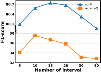
feature values well. This reduces the feature discrimination for classification. And when the number becomes a little too large, the problem of overfitting intervals is amplified.
- AutoInt takes optimal performance when K = 15 on adult and K = 10 on redwineQ, respectively. The reason might be that the instance count in the first dataset is much larger than that in the latter dataset, as shown in Table 1. As such, more numerical feature values might need more intervals to better partition the corresponding value space.
- The interval number range that makes AutoInt retain relatively good results is not small. This indicates the hyperparameter K is not very sensitive.
Effect of λ
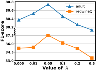
Figure 5 portrays the performance curves on adult and redwineQ as well. The results again validate the contribution of introducing soft K-means clustering to interval optimization. When λ = 0.05, the optimal results are achieved. But if we further increase λ, the performance continuously decreases and is even worse than not using the clustering loss. This is due to the reason that the effect of the main loss (classification) is weakened.
4.5 Case Study
This section conducts a case study to show how the optimized interval bounds are distributed. Two specific features are chosen as examples for illustration. The first is Age from the adult dataset and the second is pH from the whitewineQ
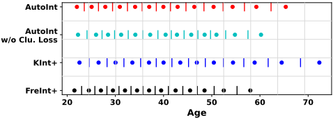
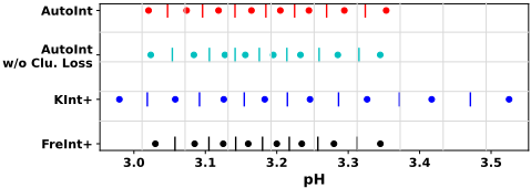
dataset. Figure 6 show the interval bounds and centres. Because the leftmost intervals and the rightmost intervals are a little too wide, we do not show them in the figure for clear visualization.
From an overall perspective, the intervals of AutoInt are distributed somewhere in between "AutoInt w/o Clu. Loss" and "KInt+". This is reasonable because the intervals of AutoInt are affected by both the classification loss and the clustering loss. On the contrary, "AutoInt w/o Clu. Loss" only uses the classification loss while "KInt+" purely performs clustering. By further comparing the interval distributions of AutoInt and "AutoInt w/o Clu. Loss", we can find AutoInt is able to let the pseudo centres become more compliant. For example, as shown in Figure 6a, the centres of the third and fourth intervals from the left are biased towards each other for "AutoInt w/o Clu. Loss". Luckily, this issue is alleviated by AutoInt, thanks to the introduction of the clustering loss.
5 RelatedWork
5.1 Logic Rule Learning
Logic rule learning is a long-standing goal in AI due to its transparency, interpretability, and reasoning ability. In the early days, template-based [Alexander and Mozer, 1994] and frequent pattern-based [Dehaspe and Toivonen, 1999] logic rule extraction methods dominate this research area. The former relies on manual endeavors for designing templates, while the latter uses frequent pattern mining algorithms and then converts frequent patterns into association rules. These rule extraction methods cannot be optimized with target objective functions.
In recent years, the trend towards fusing neural networks and logic rules continually spreads. There are two main directions: incorporating logic rules into neural networks [Hu et al., 2016; Xie et al., 2019] and using neural networks to learn logic rules [Yang et al., 2017]. This paper concentrates on the second direction. Yang et al. [2016] has performed matrix multiplications over entities in a knowledge base (KB) and derived rules from the optimized matrices. Some other studies [Dong et al., 2019; Qu et al., 2021] follow this work but all of them need relational knowledge from KBs. Similarly, Dong et al. [2019] and Glanois et al. [2022] have used neural networks to learn rules based on some background knowledge expressed in first-order logic. Some other studies use reinforcement learning [Jin et al., 2022] or evolutionary computation [Yadav et al., 2021] to learn rules.
Despite learning rules by means of neural networks, Neuro-rule networks [Wang et al., 2020] equate fullconnected neural networks with logic rules. Therefore, neural networks and logic rules share the same logical reasoning process. As aforementioned, this advantage is attributed to the novel logical layers. To improve the scalability and accuracy of Neuro-rule networks, Wang et al. [2021] have developed novel logical activation functions within logical layers and a gradient-discrete training method. Based on neuro-rule networks, Zhang et al. [2022a] have further realized personalized rule weight computation, which exhibits good performance in recommender systems.
5.2 Feature Discretization
Different from parameter binarization in neural networks [Yang et al., 2022], feature discretization [Dougherty et al., 1995] usually converts a continuous feature into a onehot vector, used for feature selection [Liu and Setiono, 1997; Sharmin et al., 2019]. The commonly-used discretization methods include equal-width interval, equal-frequency interval, etc. Decision trees [Quinlan, 2014] also largely rely on feature discretization (e.g., entropy-based methods) to construct conjunctive-form decision rules. For neurorule networks, Wang et al. [2020] have adopted an entropybased discretization method, i.e., the recursive minimal entropy partitioning algorithm, to binarize continuous features. Qiao et al. [2021] have exploited quantile discretization (i.e., equal-width interval) for binarization. Later, RRL [Wang et al., 2021] even introduces random sampling for interval bounds, hoping that NRNs will not connect unreasonable intervals with any learned rule. In contrast to the above studies, this work introduces a differentiable approach to optimize intervals together with NRNs.
6 Conclusion
In this paper, we propose an automatic continuous feature binarization approach, named AutoInt, that can serve as a basic component for neuro-rule networks. The strengths of AutoInt lie in two key modules: (1) Differentiable binarization enables the intervals to be optimized with NRNs in an end-toend manner. (2) Differentiable clustering makes the learned interval better match the original feature value distributions. The comprehensive experiments demonstrate the superiority and rationality of AutoInt. In future work, we plan to automatically learn the optimal interval number instead of setting the same number for different features.
Acknowledgments
Wei Zhang is the corresponding author. The work was supported in part by National Natural Science Foundation of China under Grant (No. 92270119, 62272264, and 62072182).
@inproceedings{ijcai2023p510,
  title     = {Learning to Binarize Continuous Features for Neuro-Rule Networks},
  author    = {Zhang, Wei and Liu, Yongxiang and Wang, Zhuo and Wang, Jianyong},
  booktitle = {Proceedings of the Thirty-Second International Joint Conference on
               Artificial Intelligence, {IJCAI-23}},
  publisher = {International Joint Conferences on Artificial Intelligence Organization},
  editor    = {Edith Elkind},
  pages     = {4584--4592},
  year      = {2023},
  month     = {8},
  note      = {Main Track},
  doi       = {10.24963/ijcai.2023/510},
  url       = {https://doi.org/10.24963/ijcai.2023/510},
}
TY - CPAPER TI - Learning to Binarize Continuous Features for Neuro-Rule Networks AU - Zhang, Wei AU - Liu, Yongxiang AU - Wang, Zhuo AU - Wang, Jianyong T2 - Proceedings of the Thirty-Second International Joint Conference on Artificial Intelligence, IJCAI-23 PB - International Joint Conferences on Artificial Intelligence Organization PY - 2023 SP - 4584 EP - 4592 DO - 10.24963/ijcai.2023/510 UR - https://doi.org/10.24963/ijcai.2023/510 ER -Copied
Machine-readable versions of this paper, for tools and AI agents:





