
pTSE: A Multi-model Ensemble Method for Probabilistic Time Series Forecasting
Proceedings of the Thirty-Second International Joint Conference on Artificial Intelligence. Main Track. Pages 4684-4692.
https://doi.org/10.24963/ijcai.2023/521
Keywords
- Machine Learning: ML: Probabilistic machine learning
- Machine Learning: ML: Time series and data streams
Abstract
Various probabilistic time series forecasting models have sprung up and shown remarkably good performance. However, the choice of model highly relies on the characteristics of the input time series and the fixed distribution that model is based on. Due to the fact that the probability distributions cannot be averaged over different models straightforwardly, the current time series model ensemble methods cannot be directly applied to improve the robustness and accuracy of forecasting. To address this issue, we propose pTSE, a multi-model distribution ensemble method for probabilistic forecasting based on Hidden Markov Model (HMM). pTSE only takes off-the-shelf outputs from member models without requiring further information about each model. Besides, we provide a complete theoretical analysis of pTSE to prove that the empirical distribution of time series subject to an HMM will converge to the stationary distribution almost surely. Experiments on benchmarks show the superiority of pTSE over all member models and competitive ensemble methods.
- [Adhikari et al., 2015] Ratnadip Adhikari, Ghanshyam Verma, and Ina Khandelwal. A model ranking based selective ensemble approach for time series forecasting. Procedia Computer Science, 48:14-21, 2015. Interna- tional Conference on Computer, Communication and Convergence (ICCC 2015).
- [Adhikari, 2015] Ratnadip Adhikari. A neural network based linear ensemble framework for time series forecast- ing. Neurocomputing, 157:231-242, 2015.
- [Akyuz et al., 2017] A. Okay Akyuz, Mitat Uysal, Berna Atak Bulbul, and M. Ozan Uysal. Ensemble approach for time series analysis in demand forecast- ing: Ensemble learning. In 2017 IEEE International Conference on INnovations in Intelligent SysTems and Applications (INISTA), pages 7-12, 2017.
- [Bilmes and others, 1998] Jeff A Bilmes et al. A gentle tu- torial of the em algorithm and its application to parameter estimation for gaussian mixture and hidden markov mod- els. International Computer Science Institute, 4(510):126, 1998.
- [Chu and Li, 2023] Zhixuan Chu and Sheng Li. Continual treatment effect estimation: Challenges and opportunities. arXiv preprint arXiv:2301.01026, 2023.
- [Chu et al., 2023] Zhixuan Chu, Ruopeng Li, Stephen Rath- bun, and Sheng Li. Continual causal inference with incremental observational data. arXiv preprint arXiv:2303.01775, 2023.
- [Faraway and Jhun, 1990] Julian J Faraway and Myoungshic Jhun. Bootstrap choice of bandwidth for density esti- mation. Journal of the American Statistical Association, 85(412):1119-1122, 1990.
- [Godahewa et al., 2021] Rakshitha Godahewa, Kasun Ban- dara, Geoffrey I Webb, Slawek Smyl, and Christoph Bergmeir. Ensembles of localised models for time se- ries forecasting. Knowledge-Based Systems, 233:107518, 2021.
- [Januschowski et al., 2020] Tim Januschowski, Jan Gasthaus, Yuyang Wang, David Salinas, Valentin Flunkert, Michael Bohlke-Schneider, and Laurent Callot. Criteria for classifying forecasting methods. Interna- tional Journal of Forecasting, 36(1):167-177, 2020. M4 Competition.
- [Koochali et al., 2021] Alireza Koochali, Andreas Dengel, and Sheraz Ahmed. If you like it, gan it-probabilistic multivariate times series forecast with gan. In Engineering Proceedings, volume 5, page 40. Multidisciplinary Digital Publishing Institute, 2021.
- [Lim et al., 2021] Bryan Lim, Sercan Ö Arık, Nicolas Lo- eff, and Tomas Pfister. Temporal fusion transformers for interpretable multi-horizon time series forecasting. Inter- national Journal of Forecasting, 2021.
- [Liu et al., 2019] Fagui Liu, Muqing Cai, Liangming Wang, and Yunsheng Lu. An ensemble model based on adaptive noise reducer and over-fitting prevention lstm for multi- variate time series forecasting. IEEE Access, 7:26102- 26115, 2019.
- [Montero-Manso et al., 2020] Pablo Montero-Manso, George Athanasopoulos, Rob J. Hyndman, and Thiyanga S. Talagala. Fforma: Feature-based forecast model averaging. International Journal of Forecasting, 36(1):86-92, 2020. M4 Competition.
- [Oliveira and Torgo, 2015] Mariana Oliveira and Luis Torgo. Ensembles for time series forecasting. In Dinh Phung and Hang Li, editors, Proceedings of the Sixth Asian Confer- ence on Machine Learning, volume 39 of Proceedings of Machine Learning Research, pages 360-370, Nha Trang City, Vietnam, 26-28 Nov 2015. PMLR.
- [Qiu et al., 2014] Xueheng Qiu, Le Zhang, Ye Ren, Pon- nuthurai N Suganthan, and Gehan Amaratunga. Ensemble deep learning for regression and time series forecasting. In 2014 IEEE symposium on computational intelligence in ensemble learning (CIEL), pages 1-6. IEEE, 2014.
- [Qiu et al., 2017] Xueheng Qiu, Ye Ren, Ponnuthurai Na- garatnam Suganthan, and Gehan A.J. Amaratunga. Em- pirical mode decomposition based ensemble deep learn- ing for load demand time series forecasting. Applied Soft Computing, 54:246-255, 2017.
- [Rangapuram et al., 2018] Syama Sundar Rangapuram, Matthias W Seeger, Jan Gasthaus, Lorenzo Stella, Yuyang Wang, and Tim Januschowski. Deep state space models for time series forecasting. Advances in neural information processing systems, 31:7785-7794, 2018.
- [Rasul et al., 2020] Kashif Rasul, Abdul-Saboor Sheikh, Ingmar Schuster, Urs Bergmann, and Roland Voll- graf. Multivariate probabilistic time series forecast- ing via conditioned normalizing flows. arXiv preprint arXiv:2002.06103, 2020.
- [Ravagli, 2021] Davide Ravagli. Mixture autoregressive models with applications to heteroskedastic time series. The University of Manchester (United Kingdom), 2021.
- [Salinas et al., 2019a] David Salinas, Michael Bohlke- Schneider, Laurent Callot, Roberto Medico, and Jan Gasthaus. High-dimensional multivariate forecasting with low-rank gaussian copula processes. arXiv preprint arXiv:1910.03002, 2019.
- [Salinas et al., 2019b] David Salinas, Valentin Flunkert, Jan Gasthaus, and Tim Januschowski. DeepAR: Probabilistic forecasting with autoregressive recurrent networks. Inter- national Journal of Forecasting, 2019.
- [Salinas et al., 2020] David Salinas, Valentin Flunkert, Jan Gasthaus, and Tim Januschowski. Deepar: Probabilistic forecasting with autoregressive recurrent networks. Inter- national Journal of Forecasting, 36(3):1181-1191, 2020.
- [Shih et al., 2019] Shun-Yao Shih, Fan-Keng Sun, and Hung-yi Lee. Temporal pattern attention for multivariate time series forecasting. Machine Learning, 108(8):1421- 1441, 2019.
- [Taylor and Letham, 2017] Sean J. Taylor and Benjamin Letham. Forecasting at scale. PeerJ Prepr., 5:e3190, 2017.
- [Wu and Yao, 2016] Qiang Wu and Weixin Yao. Mixtures of quantile regressions. Computational Statistics & Data Analysis, 93:162-176, 2016.
- [Yu et al., 2016] Hsiang-Fu Yu, Nikhil Rao, and Inderjit S Dhillon. Temporal regularized matrix factorization for high-dimensional time series prediction. In D. Lee, M. Sugiyama, U. Luxburg, I. Guyon, and R. Garnett, edi- tors, Advances in Neural Information Processing Systems, volume 29.
- Curran Associates, Inc., 2016.
- [Yuan and Kitani, 2019] Ye Yuan and Kris Kitani. Diverse trajectory forecasting with determinantal point processes. arXiv preprint arXiv:1907.04967, 2019.
References were extracted automatically from the PDF and may contain errors.
Full text extracted automatically from the PDF; figures, tables and equations may differ. The PDF is the version of record.
1 Introduction
The common requirements of time series forecasting are not only predicting the expected value of a future target, namely point estimation but also further measuring the uncertainty of the output by predicting its probability distributions, namely probabilistic forecasting. Probabilistic forecasting methods have been extensively studied in the literature, such as deterministic methods that predict the quantiles of the predictive distribution [Lim et al., 2021], probabilistic methods that sample future values from a learned approximate distribution [Salinas et al., 2020; Rangapuram et al., 2018; Salinas et al., 2019a]), and latent generative models [Yuan and Kitani, 2019; Koochali et al., 2021; Rasul et al., 2020]. These methods are usually motivated by a particular modeling focus, characterizing certain aspects of the input time series [Januschowski et al., 2020]. For instance, Prophet [Taylor and Letham, 2017] shows advantages in explicitly characterizing the fundamental time-domain components, i.e., trend and seasonality of time series, while the method in [Shih et al., 2019; Chu and Li, 2023; Chu et al., 2023] digests the frequency domain information for time series to overcome the nonstationary problem. On the other hand, the training objective of such probabilistic forecasting methods is usually maximizing a likelihood function that is conventionally assumed to be a fixed distribution, e.g., Gaussian. However, this is not always true for time series. According to [Ravagli, 2021], real world time series data is more likely to be asymmetric and multi-modal with a mixture of distributions. Both aforementioned facts bring challenges for single models. Therefore, this calls for a new way to integrate the advantages and specificity of diverse models.
To combine the advantages of different models, a popular and competitive solution is model ensemble [Oliveira and Torgo, 2015]. Generally, there are two main categories of ensemble techniques for time series. The first one learns an optimal linear combination of the predicted values returned by each member model [Akyuz et al., 2017; Adhikari, 2015] by searching for the optimal weight of each model output. The second one trains the member models as weak predictors and then combines them via a boostinglike ensemble step, where member model information, including input features, is typically required for loss reduction [Qiu et al., 2017; Liu et al., 2019; Godahewa et al., 2021; Qiu et al., 2014]. However, to the best of our knowledge, all of the aforementioned studies need to treat all member models as point estimation models, where the ensemble step handles target values not distributions, and thus cannot be directly applied to fulfill probabilistic forecasting model ensemble. In addition to such practical shortcomings, an adapted theoretical foundation aimed at a probabilistic forecasting ensemble is also highly desired.
This paper intends to fill these gaps by designing pTSE ("probabilistic time series ensemble"), a semi-parametric method, to perform distribution ensemble for probabilistic forecasting of time series. We adopt the idea from the Hidden Markov Model (HMM) to treat the collection of member models as a hidden state space, where the distribution of each observation is determined by its hidden state. Then, we incorporate "mixture quantile estimation" (MQE) into the classic Baum-Welch algorithm to estimate the distribution of model residuals, which is subsequently used to compute a distribution quantile at the prediction stage. In order to guarantee the generality, we use weighted kernel density estimation
(WKDE), a non-parametric method, to approximate the residual distributions, where the sample weight of each residual for a member model is the probability of the corresponding model in the hidden state. A bootstrap method is specifically designed to calculate the optimal bandwidth parameter for each model, which is crucial to the WKDE performance. The whole ensemble step is achieved by inferring the stationary distribution of the HMM, of which the quantile is used for forecasting. We provide a complete theoretical analysis of pTSE to prove that the empirical distribution of time series subject to an HMM will converge to the stationary distribution almost surely, and such a result is non-trivial to guess. That is to say, the whole time series approximately subjects to the stationary distribution (ensemble distribution) inferred by pTSE within any period of time. It is worth noting that pTSE takes off-the-shelf model outputs without further requiring implementation details of the member model. This makes pTSE plug-and-play and easily integrated into existing models. We evaluate pTSE on synthetic datasets to confirm the theoretical results and then on public data sets to show its superiority over single-model methods as well as ensemble methods designed for point estimation models.
The main contributions of this paper are three folds: (1) We propose pTSE, a multi-model ensemble method for probabilistic forecasting, which only takes off-the-shelf outputs from member models without requiring further information about each model; (2) We theoretically verify the ensemble distribution discovered by our method, which the time series approximately subject to within any period of time; (3) We demonstrate on real-world data sets that our ensemble method produces better performance than all member models as well as competitive point estimation model ensemble methods.
2 The pTSE Framework
In this section, we begin with giving a brief overview of HMM as a preliminary in Section 2.1. Then the core idea of pTSE is introduced in Section 2.2. The distribution evaluation procedure with a mixture quantile estimation method and its parameter selection procedure are described in Section 2.3 and Section 2.4, respectively. Section 2.5 presents the complete procedure of pTSE, including the parameter estimation stage and the prediction stage, where forecasting is made based on the ensemble distribution.
2.1 Preliminaries
We first give a brief review of HMM and then introduce its fitting process.
HMM: An HMM is a probabilistic model describing the joint probability of a collection of random variables {O1, . . . ,OT , S1, . . . , ST}[Bilmes and others, 1998]. The Ot variables, either continuous or discrete, represent the observations that we can acquire in the real world, while the St variables are hidden states corresponding to each Ot. Under an HMM, the random process {St : t ∈ N} is a Markov process satisfying
Given the state St, Ot satisfies
which demonstrates that the distribution of Ot is only determined by the hidden state.
In other words, for continuous variables, Equation (1) defines the Probability Density Function (PDF) of Ot given St, and the PDF denoted as fk(o) := p(Ot = o|St = k), is conventionally termed the "emission function".
Fitting an HMM: Fitting an HMM with a total number of K states to a dataset {Ot : t ∈ N, 1 ≤ t ≤ T} requires determining the following parameters: (1) transition matrix A = (ai,j)1≤i,j≤K of the underlying Markov process {St}, where aij = p(St+1 = j|St = i), (2) a parameter set Θ = {θk}Kk=1 of the emission function fk(o; θk), and (3) initial distribution π = (π1, . . . , πK), where πk = p(S0 = k).
The fitting is done by maximum likelihood estimation (MLE) or equivalently
However, for a dataset governed by an HMM, the undergoing state process {St : St ∈ N, 1 ≤ St ≤ K} is unknown in most cases. Therefore, the parameter estimation problem of an HMM is generally solved via an ExpectationMaximization (EM) fashion, which particularly deals with MLE problems with missing data, such as the hidden states. This EM method for fitting HMM is known as the BaumWelch algorithm [Bilmes and others, 1998].
2.2 Framework Basics
We now introduce the pTSE framework for probabilistic forecasting. A probabilistic forecasting problem usually requires to estimate the conditional distribution of yt, given a trained model M and a feature vector Xt, where Xt may contain the history of the time series along with known future information without randomness. In other words, probabilistic forecasting aims to estimate p(yt|M(Xt)).
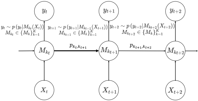
Suppose a total number of K probabilistic forecasting models, {Mk}Kk=1 , are independently fitted to the same data set {yt}Tt=1 (T ∈ N). We first assume that at each time t, there exists an optimal model Mkt ∈ {Mk}Kk=1 such that the distribution of yt is determined by the optimal model given the feature Xt. Or equivalently, yt ∼ p(yt|Mkt (Xt)).
Next, for yt+1, we assume that Mkt will randomly transfer to a new optimal model Mkt+1 with a probability of pkt,kt+1 (bold arrow in Figure 1), and this transition process is a Markov process. We illustrate this idea in Figure 1. In order to derive an executable methodology, we denote the PDF p(yt|Mkt (Xt)) as f Xt Mk (yt), for convenience.
Recall that we intend to use HMM for the model ensemble, we clarify the concepts as follows: the optimal model Mkt corresponds to the hidden state St, the time series yt corresponds to the observation Ot, and the PDF f Xt Mk (yt) corresponds to the emission function fk(o), as introduced in Section 2.1. Hence by now, we have established a framework using HMM to capture the relation between probabilistic forecasting models and the target time series.
We now introduce the method for evaluating the ensemble weights for each member model Mk. As illustrated by the law of total probability that
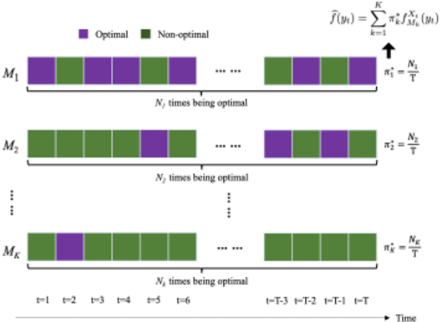
the time series subjects to an ensemble distribution of the component PDF defined by each Mk(Xt) with the weights defined as the probability of each Mk being the optimal model, i.e., p(Mk(Xt)), where Xt is a known vector without randomness. For simplicity, we estimate p(Mk(Xt)) as the average chance of Mk being the optimal model within any period of time, denoted as π∗ k , and the ensemble distribution is estimated as
We illustrate this idea in Figure 2.
Surprisingly, (π∗ 1 , . . . , π∗K ) is nothing but the stationary distribution of the hidden Markov process, which determines the expected frequency of reaching each state. For a Markov process with transition matrix A, the stationary distribution is a row vector, π∗ = (π∗ 1 , . . . , π∗K ), satisfying π∗A = π∗ , whose elements are non-negative and sum up to 1. In other words, a key step of our ensemble method is to acquire the stationary distribution of the hidden Markov process, which requires fitting an HMM to the time series {yt}Tt=1 given {Mk}Kk=1 and {Xt}Tt=1 . By substituting the variables of our interest into Equation (2), the ultimate problem we need to solve is defined as
Although it may seem to be slightly arbitrary to use the stationary distribution to evaluate the ensemble distribution, we have theoretically proved that the time series {yt : t ∈ N} approximately subject to this ensemble distribution within any period of time in Section 3.
2.3 Mixture Quantile Estimation
Generally, for a probabilistic forecasting method, the PDF f Xt Mk (yt) is not directly evaluated in the prediction stage; instead, it tends to estimate a quantile of yt, where the q-th quantile of yt is a constant τ satisfying p(yt ≤ τ) = q. Therefore, we exploit an MQE framework [Wu and Yao, 2016] to estimate Equation (3).
The MQE framework first formalizes a q-th quantile forecasting model M as y = M(X) + ϵq, where X is the vector of model inputs, and the error term ϵq is a random variable whose q-th quantile is equal to zero. Let fϵq (·) be the PDF of ϵq and the PDF of y given M(X) is fM(y) = fϵq (y -M(X)). For multiple models, the MQE framework is used to estimate the error term PDF for each model and ensure the q-th quantile of ϵq is zero for each model.
Each yt is then a random variable whose PDF is defined as f Xt Mk (yt) = f k ϵq (yt -Mk(Xt)). The function f k ϵq (·) is the error term PDF of the member model Mk and can be estimated by the MQE framework.
2.4 Kernel Density Estimation
To perform MQE, we incorporate WKDE, a non-parametric method for PDF estimation. The WKDE is used specifically to estimate the PDF of error term f k ϵq (·). A WKDE implies the importance of each sample is unequal, which in our case, is due to the diverse probabilities of different member models being the optimal model for a certain yt. The relation between sample weights and member models will be further discussed in Section 2.5.
A WKDE obtained from a dataset {yt}Tt=1 is defined as ˆ f(y) = 1 σ ∑Tt=1 wt ∑Tt=1 wtK ( y-yt σ ) ,wt > 0, where the bandwidth parameter σ essentially influences the performance. We select the optimal σ by a bootstrap method [Faraway and Jhun, 1990]. For a set of candidate bandwidth parameters Σ = {σi}, the bootstrap method first chooses an initial value σ0. Next, it constructs a total number of B sample sets by resampling from the distribution determined by a WKDE with σ0. For each σi ∈ Σ, a WKDE is performed on each resampled sample set, resulting in a PDF ˆ f bσi (·) (corresponding to the bth sample set). The selected σ∗ is the one that minimizes the bootstrap integrated mean squared error (BIMSE), or technically
In this work, we adopt the Gaussian kernel for performing WKDE. An estimated PDF f k ϵq (·) with a selected σk is denoted as f k ϵq (·; σk) for explicitness.
2.5 The MQE Baum-Welch Algorithm
We now derive the MQE Baum-Welch Algorithm for inferring both π∗ and f Xt Mk (yt) in equation 3.
Recall the problem defined in Equation 4 in Section 2.1, by MQE which refines f Xt Mk (yt) as f k ϵq (yt -Mk(Xt); σk), the objective function for the MQE Baum-Welch Algorithm is
The MQE Baum-Welch Algorithm is still an EM method for resolving Equation 6.
During the E step, four quantities αk(t), βk(t), γk(t) and ξi,j(t), need to be prepared, whose definition will be given in the following content. The E step uses the same update equations in the general Baum-Welch Algorithm introduced in [Bilmes and others, 1998]. Based on the E step, the M step is designed to update the transition matrix A, the initial distribution π, and the PDF f k ϵq (ϵ) for each member model, where the MQE method and the bootstrap procedure are performed. The EM steps are repeated until all parameters converge.
The stationary distribution π∗ in Equation (3) is obtained by setting π∗ = π and repeating π∗ = π∗A until π∗ converges, where π is the estimated initial distribution. Once π∗ and f k ϵq (ϵ) are determined, the ensemble PDF of yT+h provided with the output of each member model Mk(XT+h), i.e. ˆ f (yT+h; π∗ , f k ϵq ,Mk(XT+h)), is defined as
MQE Baum-Welch Algorithm
E step
Updating αk(t), βk(t), γk(t) and ξi,j(t): For 1 ≤ i, j ≤ K, define αk(t) and βk(t) as
and
where αk(t), βk(t) are termed forward probability and backward probability respectively.
Based on αk(t) and βk(t), γk(t) and ξi,j(t) are defined as:
which is the probability of being in state k at time t, and
which is the probability of being in state i at time t and in state j at time t + 1.
M step
Updating A and π: Each element aij of the transition matrix A is estimated as the expected number of transitions from state i to state j relative to the expected total number of transitions away from i [Bilmes and others, 1998], which is
For the initial distribution π = (π1, . . . , πK), the k-th element is estimated as the expected relative frequency in the k-th state at time 1, or
In summary, Equations (8)-(15) aim at updating the transition matrix A and the initial distribution π, with f k ϵq (ϵ) fixed.
Selecting σk for f k ϵq (ϵ): Our MQE method subsequently updates the emission function or the PDF f k ϵq (ϵ). It first selects a bandwidth parameter σk for each f k ϵq (ϵ) via the bootstrap method. In the bootstrap procedure, γk(t) is used as the sample weight of each ϵtk , where ϵtk = yt -Mk(Xt). We use γk(t) as sample weight because it is the probability of Mk being the hidden state of yt [Bilmes and others, 1998]. Therefore, for each member model, samples with larger probability should be paid more attention to.
Updating f k ϵq (ϵ) by MQE: Based on σk, a simple weighted-KDE-like update equation for f k ϵq (ϵ) would be ∑Tt=1 γk(t) σk ∑t γk(t) K ( ϵ-ϵtk σk ). However, this update equation ignores which quantile is being estimated by the member models. To make the method focus on the q-th quantile, f k eq (ϵ) is updated as
where Ikt,1 = I{ϵtk≤0} 1 and Ikt,2 = I{ϵtk>0} [Wu and Yao, 2016]. The constants W k 1 and W k 2 constrain f k ϵq (ϵ) to have 0 as the q-th quantile, while normalizing the integral of f k ϵq (ϵ) equal to 1. By defining vk,t = ∫ 0-∞ 1 σk K ( ϵ-ϵtk σk ) dϵ, W k 1
1 The indicator function I{·} is a 0/1 valued function, which is defined as I{c} = 1 if c is true, and 0 otherwise.
and W k 2 are acquired by solving the following linear equation systems,
Prediction Step
Once the learning procedure stops, the q-th quantile τ at time T + h is obtained by solving Equation (16)
Therefore, the future q-th quantile for a time series is estimated from ensemble PDF with Equation (16) and can be directly used at the prediction stage.
3 Theoretical Analysis
In this section, we present the theoretical results of our work. The core idea is to evaluate the limit of the empirical distribution of a sample set originated by an HMM. The results are non-trivial because a random process {Ot}+∞ t=0 generated from an HMM is not necessarily a Markov process. Strictly speaking, Equation (17) is not always equal to Equation (18) for a given initial distribution π, where F(o) = (f1(o), . . . , fK(o))T and fk(o) is the emission function as introduced in 2.1.
We summarize our theoretical work in four lemmas and one theorem. Lemma 3.1 is a straightforward statement of the property of a transition matrix. Both Lemma 3.2 and Lemma 3.3 illustrate convergence. Lemma 3.2 computes the final limit with the help of Lemma 3.1. Lemma 3.3 assures the existence of the limit of the sum of a random variable sequence, providing fast dependence decay. Lemma 3.4, indicating the exponential convergence rate of a Markov Process, turns out to be a guarantee for the condition in Lemma 3.3. Remarkably, based on Lemma 3.1-3.4, Theorem 3.1 indicates that the empirical distribution of a dataset sampled from an HMM converges to ∑Kk=1 π∗ k fk(o) almost surely. In other words, these HMM samples are approximately subject to an ensemble distribution of the emission functions, fk(o), with the weights determined by the stationary distribution regardless of the time window. In the case of pTSE, each emission function fk(yt) is defined as f k ϵq (yt -Mk(Xt)). Hence as a corollary, within any period of time, the time series {yt : t ∈ N} approximately subjects to the ensemble distribution in Equation (7), estimated by the MQE Baum-Welch Algorithm.
Lemma 3.1. Let A be the transition probability matrix of an HMM, and let
then 1 is a right eigenvector of eigenvalue 1 of A, i.e.
The proof is straightforward.
Lemma 3.2. Let A be the transition probability matrix of an HMM, π∗ be the stationary distribution, and π be any initial distribution, let F(o) be the vector-valued emission function of all states, then
Lemma 3.3. Let {En : n ≥ 1} be a sequence of events and Sn = ∑nk=1 IEk , if there exists {ρn}∞n=1 satisfying ∑n |ρn| ≤ +∞, such that, for any i ̸= j,
and if limn→+∞E(Sn) = +∞,then,
Lemma 3.4. Let A be the transition probability matrix of a Markov Process with non-zero elements and π∗ be the stationary distribution. Then, there exists a constant C, such that the following inequality holds,
| (A) | Traffic | Electric | Solar Energy | ||||||
|---|---|---|---|---|---|---|---|---|---|
| Model | 0.5-risk | 0.9-risk | AVG | 0.5-risk | 0.9-risk | AVG | 0.5-risk | 0.9-risk | AVG |
| DeepAR | 0.151 | 0.302 | 0.227 | 0.083 | 0.070 | 0.076 | 0.435 | 0.253 | 0.344 |
| SFF | 0.235 | 0.471 | 0.353 | 0.084 | 0.047 | 0.066 | 0.509 | 0.278 | 0.393 |
| TFT | 0.184 | 0.367 | 0.275 | 0.118 | 0.062 | 0.090 | 0.487 | 0.184 | 0.336 |
| Transformer | 0.163 | 0.326 | 0.244 | 0.087 | 0.058 | 0.072 | 0.499 | 0.270 | 0.385 |
| pTSE (Ours) | 0.150 | 0.106 | 0.128 | 0.079 | 0.042 | 0.061 | 0.451 | 0.210 | 0.331 |
| (B) | Traffic | Electric | Solar Energy | ||||||
| Model | 0.5-risk | 0.9-risk | AVG | 0.5-risk | 0.9-risk | AVG | 0.5-risk | 0.9-risk | AVG |
| ModelRank | 0.150 | 0.108 | 0.129 | 0.073 | 0.049 | 0.061 | 0.457 | 0.210 | 0.334 |
| FFORMA | 0.165 | 0.112 | 0.139 | 0.081 | 0.070 | 0.076 | 0.459 | 0.284 | 0.372 |
| pTSE (Ours) | 0.150 | 0.106 | 0.128 | 0.079 | 0.042 | 0.061 | 0.451 | 0.210 | 0.331 |
where J is the size of the largest Jordan block of A, and λt-J+1 ∗ is the largest absolute value of the eigenvalues smaller than 1 of A. || · ||F is the Frobenius Norm.
Theorem 3.1. Let {Ot}Tt=1 be the observations generated from an HMM whose transition matrix has non-zero elements, π∗ be the stationary distribution, and F(o) be the vectorvalued emission function of all states. Define ˆ FT (τ), the empirical distribution of {Ot}Tt=1 , as
then,
4 Numerical Experiments
In this section, we first present a few synthetic data experiments to verify our theoretical results. Next, we apply the pTSE to publicly available datasets to test the performance.
4.1 Synthetic Data Analysis
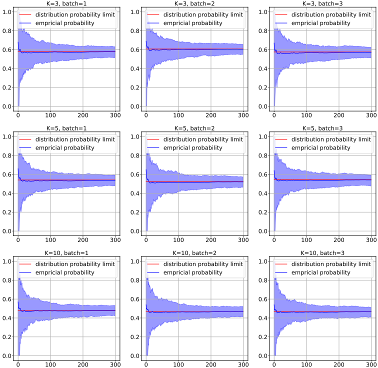
We simulated random sequences governed by HMM structures. We set K = 3, 5, 10 and T = 1000. The transition matrix A is chosen by first generating a matrix of uniformly distributed random numbers and then normalizing the matrix to ensure the sum of elements of each row equals 1. The emission function fk(o) for each state k is simply set to a Gaussian distribution as N(0.2k, √k + 1), (k = 1, . . . ,K). For each set of {K, T,A,F(o)}, we run the simulation procedure for 100 times, where during each time, an initial distribution π0 is randomly chosen. The results are presented in Figure 3. The empirical probability, ˆ F(τ), shows fast convergence to π∗ ∫ τ-∞ F(o)do, after T = 50 for all simulated datasets, regardless of the state number K or the transition matrix A.
4.2 Real World Data Analysis
We evaluate the performance of pTSE on three challenging real-world benchmark datasets, i.e., solar energy 2 , electricity, traffic [Yu et al., 2016].The solar energy, electricity, and traffic datasets contain hourly measurements from 137, 370, and 963 time series, respectively. For these three datasets, each model would perform an iterative prediction task of forecasting the future values for a 24-hour horizon after being trained on the past 168-hour (past week) data. The model performance would be evaluated on a 7-day-horizon test set.
2 https://www.nrel.gov/grid/solar-power-data.html
Four of the most popular probabilistic forecasting models are selected as the member models: SimpleFeedForwardEstimator (SFF), Transformer, DeepAR, and TemporalFusionTransformer (TFT). As in [Salinas et al., 2019b], we use qrisk metrics (quantile loss) to quantify the accuracy of a q-th quantile of the predictive distribution. Table 1 presents 0.5risk, 0.9-risk, and the average risk of the output corresponding to each method. We also present a comparison of pTSE with existing time series model ensemble methods, FFORMA [Montero-Manso et al., 2020], a meta-learning approach, and a model ranking-based ensemble method [Adhikari et al., 2015]. Hyperparameters of the two ensemble methods are set up as recommended in the original papers. Results in Table 1 show that pTSE outperforms all member models on average across all datasets. The performance of pTSE is relatively more stable in the electricity and traffic datasets, as it ranked highest in all three competitions in each case. On the solar energy dataset, pTSE maintained the best performance in the average loss. Compared with the other two ensemble methods, pTSE shows a significant advantage on three datasets.
5 Conclusion
We present pTSE, a semi-parametric multi-model ensemble methodology for probabilistic forecasting. Our method takes off-the-shelf model outputs without requiring further information. We theoretically prove the empirical distribution of time series subject to an HMMwill converge to the stationary distribution almost surely. We use the synthetic data to verify the validity of our theory and conduct extensive experiments on three benchmark datasets to demonstrate the superiority of pTSE over each member model and other model ensemble methods. Nevertheless, it should be pointed out that the improvement by pTSE or any other ensemble methods is essentially limited by the performance of member models.
@inproceedings{ijcai2023p521,
  title     = {pTSE: A Multi-model Ensemble Method for Probabilistic Time Series Forecasting},
  author    = {Zhou, Yunyi and Chu, Zhixuan and Ruan, Yijia and Jin, Ge and Huang, Yuchen and Li, Sheng},
  booktitle = {Proceedings of the Thirty-Second International Joint Conference on
               Artificial Intelligence, {IJCAI-23}},
  publisher = {International Joint Conferences on Artificial Intelligence Organization},
  editor    = {Edith Elkind},
  pages     = {4684--4692},
  year      = {2023},
  month     = {8},
  note      = {Main Track},
  doi       = {10.24963/ijcai.2023/521},
  url       = {https://doi.org/10.24963/ijcai.2023/521},
}
TY - CPAPER TI - pTSE: A Multi-model Ensemble Method for Probabilistic Time Series Forecasting AU - Zhou, Yunyi AU - Chu, Zhixuan AU - Ruan, Yijia AU - Jin, Ge AU - Huang, Yuchen AU - Li, Sheng T2 - Proceedings of the Thirty-Second International Joint Conference on Artificial Intelligence, IJCAI-23 PB - International Joint Conferences on Artificial Intelligence Organization PY - 2023 SP - 4684 EP - 4692 DO - 10.24963/ijcai.2023/521 UR - https://doi.org/10.24963/ijcai.2023/521 ER -Copied
Machine-readable versions of this paper, for tools and AI agents:





