
A Diffusion Model with Contrastive Learning for ICU False Arrhythmia Alarm Reduction
Proceedings of the Thirty-Second International Joint Conference on Artificial Intelligence. Main Track. Pages 4912-4920.
https://doi.org/10.24963/ijcai.2023/546
Keywords
- Multidisciplinary Topics and Applications: MDA: Health and medicine
- Machine Learning: ML: Applications
- Machine Learning: ML: Time series and data streams
Abstract
The high rate of false arrhythmia alarms in intensive care units (ICUs) can negatively impact patient care and lead to slow staff response time due to alarm fatigue. To reduce false alarms in ICUs, previous works proposed conventional supervised learning methods which have inherent limitations in dealing with high-dimensional, sparse, unbalanced, and limited data. We propose a deep generative approach based on the conditional denoising diffusion model to detect false arrhythmia alarms in the ICUs. Conditioning on past waveform data of a patient, our approach generates waveform predictions of the patient during an actual arrhythmia event, and uses the distance between the generated and the observed samples to classify the alarm. We design a network with residual links and self-attention mechanism to capture long-term dependencies in signal sequences, and leverage the contrastive learning mechanism to maximize distances between true and false arrhythmia alarms. We demonstrate the effectiveness of our approach on the MIMIC II arrhythmia dataset for detecting false alarms in both retrospective and real-time settings.
- [Aboukhalil et al., 2008] Anton Aboukhalil, Larry Nielsen, Mohammed Saeed, Roger G Mark, and Gari D Clifford. Reducing false alarm rates for critical arrhythmias using the arterial blood pressure waveform. Journal of biomedi- cal informatics, 41(3):442-451, 2008.
- [Alcaraz and Strodthoff, 2022] Juan Miguel Lopez Alcaraz and Nils Strodthoff. Diffusion-based time series impu- tation and forecasting with structured state space models. arXiv preprint arXiv:2208.09399, 2022.
- [Ansari et al., 2015] Sardar Ansari, Ashwin Belle, and Kay- van Najarian. Multi-modal integrated approach towards reducing false arrhythmia alarms during continuous pa- tient monitoring: the physionet challenge 2015. In 2015 Computing in Cardiology Conference (CinC), pages 1181-1184. IEEE, 2015.
- [Bashar and Nayak, 2020] Md Abul Bashar and Richi Nayak. Tanogan: Time series anomaly detection with generative adversarial networks. In 2020 IEEE Sympo- sium Series on Computational Intelligence (SSCI), pages 1778-1785. IEEE, 2020.
- [Behar et al., 2014] Joachim Behar, Julien Oster, and Gari D Clifford. Combining and benchmarking methods of foetal ecg extraction without maternal or scalp electrode data. Physiological measurement, 35(8):1569, 2014.
- [Caballero and Mirsky, 2015] Miguel Caballero and Grace M Mirsky. Reduction of false cardiac arrhythmia alarms through the use of machine learning techniques. In 2015 Computing in Cardiology Conference (CinC), pages 1169-1172. IEEE, 2015.
- [Clifford et al., 2015] Gari D Clifford, Ikaro Silva, Benjamin Moody, Qiao Li, Danesh Kella, Abdullah Shahin, Tristan Kooistra, Diane Perry, and Roger G Mark. The phys- ionet/computing in cardiology challenge 2015: reducing false arrhythmia alarms in the icu. In 2015 Computing in Cardiology Conference (CinC), pages 273-276. IEEE, 2015.
- [Couto et al., 2015] Paula Couto, Ruben Ramalho, and Rui Rodrigues. Suppression of false arrhythmia alarms using ecg and pulsatile waveforms. In 2015 Computing in Car- diology Conference (CinC), pages 749-752. IEEE, 2015.
- [Deng et al., 2021] Jinliang Deng, Xiusi Chen, Renhe Jiang, Xuan Song, and Ivor W Tsang. St-norm: Spatial and tem- poral normalization for multi-variate time series forecast- ing. In Proceedings of the 27th ACM SIGKDD conference on knowledge discovery & data mining, pages 269-278, 2021.
- [Eerikäinen et al., 2015] Linda M Eerikäinen, Joaquin Van- schoren, Michael J Rooijakkers, Rik Vullings, and Ronald M Aarts. Decreasing the false alarm rate of ar- rhythmias in intensive care using a machine learning ap- proach. In 2015 Computing in Cardiology Conference (CinC), pages 293-296. IEEE, 2015.
- [Engelse and Zeelenberg, 1979] Willem AH Engelse and Cees Zeelenberg. A single scan algorithm for qrs- detection and feature extraction. Computers in cardiology, 6(1979):37-42, 1979.
- [Fallet et al., 2015] Sibylle Fallet, Sasan Yazdani, and Jean- Marc Vesin. A multimodal approach to reduce false ar- rhythmia alarms in the intensive care unit. In 2015 Com- puting in Cardiology Conference (CinC), pages 277-280. IEEE, 2015.
- [Goodfellow et al., 2020] Ian Goodfellow, Jean Pouget- Abadie, Mehdi Mirza, Bing Xu, David Warde-Farley, Sherjil Ozair, Aaron Courville, and Yoshua Bengio. Gen- erative adversarial networks. Communications of the ACM, 63(11):139-144, 2020.
- [He et al., 2016] Kaiming He, Xiangyu Zhang, Shaoqing Ren, and Jian Sun. Deep residual learning for image recog- nition. In Proceedings of the IEEE conference on computer vision and pattern recognition, pages 770-778, 2016.
- [He et al., 2020] Kaiming He, Haoqi Fan, Yuxin Wu, Sain- ing Xie, and Ross Girshick. Momentum contrast for unsu- pervised visual representation learning. In Proceedings of the IEEE/CVF conference on computer vision and pattern recognition, pages 9729-9738, 2020.
- [Ho et al., 2020] Jonathan Ho, Ajay Jain, and Pieter Abbeel. Denoising diffusion probabilistic models. Advances in Neural Information Processing Systems, 33:6840-6851, 2020.
- [Hooman et al., 2018] Oroojeni MJ Hooman, Moham- mad Majid Al-Rifaie, and Mihalis A Nicolaou. Deep neuroevolution: Training deep neural networks for false alarm detection in intensive care units. In 2018 26th European Signal Processing Conference (EUSIPCO), pages 1157-1161. IEEE, 2018.
- [Kalidas and Tamil, 2016] V Kalidas and LS Tamil. Cardiac arrhythmia classification using multi-modal signal analy- sis. Physiological measurement, 37(8):1253, 2016.
- [Kingma and Welling, 2013] Diederik P Kingma and Max Welling. Auto-encoding variational bayes. arXiv preprint arXiv:1312.6114, 2013.
- [Kong et al., 2020] Zhifeng Kong, Wei Ping, Jiaji Huang, Kexin Zhao, and Bryan Catanzaro. Diffwave: A versa- tile diffusion model for audio synthesis. arXiv preprint arXiv:2009.09761, 2020.
- [Krasteva et al., 2015] V Krasteva, Irena Jekova, Remo Leber, Ramun Schmid, and Roger Abächerli. Validation of arrhythmia detection library on bedside monitor data for triggering alarms in intensive care. In 2015 Computing in Cardiology Conference (CinC), pages 737-740. IEEE, 2015.
- [Lawless, 1994] Stephen T Lawless. Crying wolf: false alarms in a pediatric intensive care unit. Critical care medicine, 22(6):981-985, 1994.
- [Lehman et al., 2018] Eric P Lehman, Rahul G Krishnan, Xiaopeng Zhao, Roger G Mark, and H Lehman Li-Wei. Representation learning approaches to detect false arrhyth- mia alarms from ecg dynamics. In Machine learning for healthcare conference, pages 571-586. PMLR, 2018.
- [Mousavi et al., 2020] Sajad Mousavi, Atiyeh Fotoohinasab, and Fatemeh Afghah. Single-modal and multi-modal false arrhythmia alarm reduction using attention-based convolutional and recurrent neural networks. PloS one, 15(1):e0226990, 2020.
- [Nygårds and Sörnmo, 1983] M-E Nygårds and L Sörnmo. Delineation of the qrs complex using the envelope of the ecg. Medical and biological engineering and computing, 21(5):538-547, 1983.
- [Oster et al., 2013] Julien Oster, Joachim Behar, Roberta Colloca, Qichen Li, Qiao Li, and Gari D Clifford. Open source java-based ecg analysis software and android app for atrial fibrillation screening. In Computing in Cardiol- ogy 2013, pages 731-734. IEEE, 2013.
- [Pan and Tompkins, 1985] Jiapu Pan and Willis J Tompkins. A real-time qrs detection algorithm. IEEE transactions on biomedical engineering, (3):230-236, 1985.
- [Parthasarathy and Tobin, 2009] Sairam Parthasarathy and Martin J Tobin. Sleep in the intensive care unit. Applied Physiology in Intensive Care Medicine, pages 191-200, 2009.
- [Plesinger et al., 2015] Filip Plesinger, Petr Klimes, Josef Halamek, and Pavel Jurak. False alarms in intensive care unit monitors: detection of life-threatening arrhyth- mias using elementary algebra, descriptive statistics and fuzzy logic. In 2015 Computing in Cardiology Conference (CinC), pages 281-284. IEEE, 2015.
- [Sadr et al., 2015] Nadi Sadr, Jacqueline Huvanandana, Doan Trang Nguyen, Chandan Kalra, Alistair McEwan, and Philip de Chazal. Reducing false arrhythmia alarms in the icu by hilbert qrs detection. In 2015 Computing in Cardiology Conference (CinC), pages 1173-1176. IEEE, 2015.
- [Tashiro et al., 2021] Yusuke Tashiro, Jiaming Song, Yang Song, and Stefano Ermon. Csdi: Conditional score- based diffusion models for probabilistic time series impu- tation. Advances in Neural Information Processing Sys- tems, 34:24804-24816, 2021.
- [Vaswani et al., 2017] Ashish Vaswani, Noam Shazeer, Niki Parmar, Jakob Uszkoreit, Llion Jones, Aidan N Gomez, Łukasz Kaiser, and Illia Polosukhin. Attention is all you need. Advances in neural information processing systems, 30, 2017.
- [Wang et al., 2022] Zhendong Wang, Huangjie Zheng, Pengcheng He, Weizhu Chen, and Mingyuan Zhou. Diffusion-gan: Training gans with diffusion, 2022.
- [Yu et al., 2021] Qiang Yu, Cheng Wang, Jing Xi, Ying Chen, Weifeng Li, Yun Ge, and Xiaolin Huang. Intensive care unit false alarm identification based on convolution neural network. IEEE Access, 9:81841-81854, 2021.
- [Zhou et al., 2019] Bin Zhou, Shenghua Liu, Bryan Hooi, Xueqi Cheng, and Jing Ye. Beatgan: Anomalous rhythm detection using adversarially generated time series. In IJ- CAI, pages 4433-4439, 2019. IJCAI
- [Zhou et al., 2022] Yuerong Zhou, Guoshuai Zhao, Jun Li, Gan Sun, Xueming Qian, Benjamin Moody, Roger G Mark, and Li-wei H Lehman. A contrastive learning ap- proach for icu false arrhythmia alarm reduction. Scientific reports, 12(1):1-10, 2022.
- [Zong et al., 2003] W Zong, GB Moody, and D Jiang. A ro- bust open-source algorithm to detect onset and duration of qrs complexes. In Computers in Cardiology, 2003, pages 737-740. IEEE, 2003.
References were extracted automatically from the PDF and may contain errors.
Full text extracted automatically from the PDF; figures, tables and equations may differ. The PDF is the version of record.
1 Introduction
Intensive care units (ICUs) provide care for the most vulnerable and medically unstable patients within the hospital setting. By utilizing advanced bedside monitors like electrocardiogram (ECG), arterial blood pressure (ABP) catheter and pulse oximeter (PPG), clinical staff can closely monitor the patient's physiological indicators and get alerts from the monitors when certain indicators exceed thresholds. However, ICU false alarm rate is as high as 86%; between 6% and 40% of alarms are true alarms but requiring no immediate action, and only 2% to 9% of alarms are important and useful for the medical care [Lawless, 1994]. The low ICU true alarm rate brings stress and noise for both patients and medical staff, leading to decreased quality of patient care and longer stays in the ICUs [Parthasarathy and Tobin, 2009]. Therefore, the false alarms present an important open problem in the ICUs. According to the PhysioNet Challenge in 2015, among all of the life-threatening arrhythmia alarms, ventricular tachycardia and ventricular flutter/fibrillation have proven to be the most challenging false arrhythmia alarms to detect.
Prior to the development of the deep learning methods, signal processing and conventional machine learning techniques have been developed for detecting false alarm in the ICUs through a combination of feature engineering and expertdefined rules. Such methods generally consist of a feature extractor based on different methods (including digital filtering [Pan and Tompkins, 1985; Engelse and Zeelenberg, 1979], length transform [Zong et al., 2003] and peak energy detector [Nyg˚ards and S¨ornmo, 1983; Oster et al., 2013; Behar et al., 2014]) and rule-based logics analysis. In fact, the best-performing methods from Challenge 2015 was based on a series of decision rules designed by experts [Plesinger et al., 2015]. These rules include pulse detection [Ansari et al., 2015], QRS detection [Couto et al., 2015; Sadr et al., 2015], heart rate and spectral purity values [Fallet et al., 2015], noise detection. While rule-based approaches often deliver promising results, they rely on expert-derived rule designs and good data qualities. These approaches are time consuming to develop requiring domain knowledge, sensitive to changes in complex patterns of waveform data, and often requiring significant manual adjustment of the algorithm before they can be applied to new datasets.
In recent years, there has been growing interest in machine learning and deep learning methods to detect the false alarms in ICUs. Deep learning methods use convolutional neural networks or recurrent neural networks to encode information from different channels. For example, Zhou et al. design a convolutional neural network (CNN) to discriminate between true and false alarms [Zhou et al., 2022]. The method utilizes Contrastive Learning to simultaneously minimize a binary cross entropy classification loss and a proposed similarity loss from pair-wise comparisons of waveform segments over time as a discriminative constraint. Despite the remarkable feature extraction and representation learning capabilities of deep learning methods, their performance can be hindered by several challenges, including limited samples, unbalanced labels, and sparse data.
In this paper, we develop a novel deep generative approach using diffusion modeling [Ho et al., 2020] and contrastive learning to detect false arrhythmia alarms in the ICUs. Due to the fact that false arrhythmia alarms can be triggered by various causes, the resulting waveforms can exhibit substantial variation. The main idea of our proposed model is to generate the "true" alarm waveform segment (the physiological waveform that occur in actual arrhythmia events) conditioned on the patient's past waveform data and compare the generated waveform predictions with the actual observed waveform. If the candidate observed sample is from a genuine arrhythmia alarm, the distance between the generated waveforms and the observed samples will be small; on the other hand, if the alarm is false, the discrepancy between the two will be large. We use the diffusion model as our generative model. However, the original diffusion model cannot generate the conditional distribution. Inspired by Yusuke et al. [Yu et al., 2021] and Kong et al. [Kong et al., 2020], we utilize the conditional score-based diffusion model and separate the input into observations and reconstruction target, and we designed the network with residual link [He et al., 2016] and transformer [Vaswani et al., 2017] structure to serve as the denoise process in the diffusion model. Moreover, we also introduce a contrastive learning mechanism to minimize the mutual information between the true arrhythmia signal and the false, which helps the model train better. In the inference process, we generate the true arrhythmia signal with candidates' features by the well-trained conditional diffusion model, and determine the false alarm by the distance between the generated waveform and the sample waveform. Our approach requires only a single type of samples for training, side-stepping the problems encountered in the deep models described above. We also note that our model is formulated for time series prediction tasks or anomaly detection tasks, and is not restricted to the arrhythmia alarm classification.
Our main contributions are as follows:
- We propose a diffusion model-based architecture for arrhythmia detection. Compared with the generative models of GAN and VAE, our model is easier to train and more stable. To the best of our knowledge, we are the first to apply the diffusion model to the field of ICU alarm determination or anomaly detection.
- We incorporated a contrastive learning framework into the conditional diffusion model to improve the quality and accuracy of model generation.
- We propose a novel network structure to enhance the feature capture capability of the conditional diffusion model for long time series, and is competitive with existing baselines designed for these tasks.
2 RelatedWork
ICU false alarm detection. In order to reduce the false alarms in ICUs, an extensive number of approaches have been proposed in this field. Typically, they fall into three general categories: 1) Rule-based method, detecting false alarms based on the rules defined by experts. These methods often utilize signal processing algorithms to improve the quality of observed signals. For example, Krasteva et al. use an expert database including modules for lead quality monitoring, heartbeat detection, heartbeat classification and ventricular fibrillation detection to support the decision module for final alarm inspection [Krasteva et al., 2015]; 2) Traditional machine learning based method, such as supported vector machine (SVM) [Kalidas and Tamil, 2016], decision trees [Caballero and Mirsky, 2015] and random forest [Eerik¨ainen et al., 2015], extracting important features from the arrhythmia signals to enhance detection of false alarm. Hooman et al. present a neuroevolution based-approach for training neural networks based on genetic algorithms, reducing the number of suppressed true alarms by deploying and adapting Dispersive Flies Optimisation (DFO) [Hooman et al., 2018]. Mohammad et al. utilize a low-computational gametheoretic feature selection method based on the genetic algorithm to collect information from various monitoring devices [Mousavi et al., 2020]; 3) Deep learning based method, by apply neural networks such as CNN, LSTM, and attention mechanism based network for enhancing the capability of learning representation of signals. Lehman et al. propose a supervised denoising autoencoder model utilizing the FFTtransform to process waveform data at a beat-by-beat basis [Lehman et al., 2018]. Yu et al. propose two network structures deep group convolutional neural network (DGCN) and embedded deep group convolutional network (EDGCN) to deal with different signal channels [Yu et al., 2021].
Diffusion model. Diffusion models [Ho et al., 2020] have emerged as a powerful new family of deep generative models that are prominent in many areas such as text-image generation, video generation, and molecular design. Compared to other generative models such as GAN [Goodfellow et al., 2020], VAE [Kingma and Welling, 2013] and autoregressive models, diffusion models have the advantages of being easy to train, stable, versatile and flexible [Wang et al., 2022]. Recently, diffusion models have also been applied to the task of sequence data generation. Kong et al. propose a denoising diffusion model to generate high-fidelity audio and achieve better performance than GAN-based models and Autoregressive models [Kong et al., 2020]. Tashiro et al. present a novel time series imputation method that leverages score-based diffusion models, exploiting correlations within temporal data and adopt the form of self-supervised training to optimize the diffusion models [Tashiro et al., 2021].
3 Methodology
3.1 Denoising Diffusion Probabilistic Models
Diffusion models learn a mapping from latent space to signal space by sequentially learning to remove noise in a backward process. It makes use of two Markov chains: a forward chain that perturbs data to noise, and a reverse chain that converts noise back to data. New data points are subsequently generated by first sampling a random vector from the prior distribution, followed by ancestral sampling through the reverse Markov chain. The forward process is parameterized as:
where q(xt|xt-1) is a transition kernel, which is usually designed as Gaussian perturbation and obey N(xt; √1-βtxt-1, βtI). The βt is a small positive constant that represents a noise level. xt can be expressed in closed form as:
where ˆα := 1 - βt and αt := ∏ti=1 ˆαi. Then xt can be expressed as xt = √αtx0 + (1 - αt) ε, where ε ∼ N(0, I). When α ≈ 0, xT is close to the Gaussian distribution.
Briefly speaking, this forward process slowly injects noise into the data until the data becomes completely noisy. In contrast, we need a denoising process to gradually noise down noisy data into usable data by a learnable Markov chain. Specifically, the reverse Markov chain is parameterized by a prior distribution p(xT ) = N(xt; 0, I) and a learnable transition kernel pθ(xt-1|xt). Where prior distribution can be constructed due to the conclusion of forward process, and the transition kernel can take the form of:
where θ denotes the model parameters, learned by deep neural networks. According to Ho et al. proposed denoising diffusion probabilistic models [Ho et al., 2020], µθ(xt, t) and σ(xt, t) can be parameterized as:
Then, we can calculate the parameter θ by training the following objective:
After training, we can get sample x0 from the transition kernel pθ(xt-1|xt). Since we need to generate signals conditional on the candidate samples, the existing diffusion model can only generate unconditional samples. Therefore, we need to extend the model to a form with conditional generation. Tashiro et al.[Tashiro et al., 2021] and Alcaraz et al. [Alcaraz and Strodthoff, 2022] propose a conditional diffusion process, which is, given a sample x0 which contains conditional part xc0 ∈ x0 and generation target part xg0 ∈ x0, the generated objective becomes to predict the target data distribution when the conditional data distribution is known, i.e., the forward process q(xg0 |xc0 ) and the denoising process p(xg0 |xc0 ). Due to the pθ(x0:T ) can be defined as the trained model pθ(x0), similarly, we can extend the denoising process to the conditional case by introducing xg0 and xc0 to Eq.3 and Eq.4:
where xgT N(0, I). Now, we can use deep neural networks to simulate the reverse process. As in Alcaraz et al[Alcaraz and Strodthoff, 2022], we train the conditional observation data, time dimension, and noise space as the input of the neural network to get the appropriate function to simulate the inverse process performed.
3.2 Model Architecture
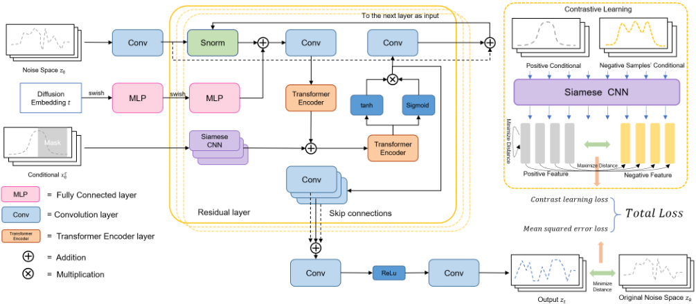
In this section, we present a variant of the Diffwave-based diffusion model. The model's architecture is depicted schematically in Figure 1. The inputs of our model include Noise Space z0, Diffusion Embedding t and Conditional Observation Data xc0 . Then we utilize a network with residual link structure to get the trained θ for the denoising process.
Diffusion Embedding. It is important to include the diffusion-step t as part of the input, as the model need to embed the time step information for modeling the pθ(xg0 |xc0 ) → pθ(xgT |xc0 ). we use the following 128-dimensions embedding following previous works[Kong et al., 2020]:
Then we apply two MLP layers to encode the time embedding information. The first MLP layer is outside of the residual layer for sharing parameters. The second MLP layer is integrated into residual layers for adjusting the shape, which makes time embedding can map into the input of each residual layer.
Residual layer. Both residual and skip connections are used throughout the network, to speed up convergence and enable training of much deeper model. Firstly, we use the spatial normalization network (S-norm) [Deng et al., 2021] to process inputs of residual layer, which enable the model to capture fine-grained variation by distilling the local or highfrequency components from the observed signal. Then, the processed noise z0 is added to the time embedding t, which is processed and fed into the feature extraction module:
where InputT1 is input of the first transformer encoder layer. SN(·) means S-norm layer. We choose the transformer encoder as our feature extractor because the self-attentive mechanism has a good ability to model long sequences and capture the temporal and spatial dependencies in multivariate time series. After the encoder layer, we get the representation X1 en of noise and time embedding.
Also, we need to extract the features of the conditional observations to guide the diffusion model to generate the desired time series. Since this feature extractor needs to exist in the residual layer, we chose a 1-layer convolutional neural network to extract the features of the conditional data. Meanwhile, as we need to employ this CNN to extract features of conditional samples in the contrastive learning module, we name it Siamese CNN. The hidden representation of the conditional observation data will be added to the result of the first transformer encoder as the input to the second transformer encoder:
where xc0 is conditional observation data. X2 en means the output of the second transformer encoder. We deploy a gated activation unit and get final output:
where × denotes a convolution operator, ⊙ denotes an element-wise multiplication operator. σ· and tanh denote sigmoid function and tanh function, respectively. Wf and Wg are learnable convolution filters. Finally, z is split into two parts, each after passing through a learnable convolutional layer, as the input to the next residual layer and part of the total output of the residual module, respectively.
3.3 Contrastive Learning and Loss Function
To generate higher quality candidate samples, we introduced Contrastive Learning mechanism into conditional denoise diffusion model to improve the likelihood of the model generating positive samples. Specifically, we use Siamese CNN to extract the features of positive and negative samples, respectively. We introduce a set of negative hidden representation H′ = h′1 , h′2 ...h′n′ , which is encoded from n′ negative samples XN = xN1 , xN2 , ..., xNn′ . Conversely, the positive hidden representations H = h1, h2...hn also are encoded from n positive samples XP = xP1 , xP2 , ..., xPn ,
Then, we can use a contrastive learning loss to maximize the distance between the features of positive and negative samples. In the alarm classification task, we want the model to generate waveforms that are closer to the waveforms of real alarms and away from the waveforms of false alarms. Therefore, we use only real arrhythmia waveform data during training and they are marked as positive samples. We sample from waveforms that are labeled as false alarms as negative samples. We choose InfoNCE loss [He et al., 2020] as our contrastive loss function LC in this paper:
where n denotes the number of samples, h′ and h denote features from negative samples and postive samples, respectively. As we only want to amplify the distance between the positive and negative sample features, we use the positive sample itself to reduce the impact in the numerator. Ideally, we would like a positive sample to compute the distance with all the negative samples, but this would incur an unaffordable computational overhead. Hence we can only sample n samples from the entire negative sample space for the calculation of the contrastive learning loss.
Since in the conditional diffusion model, pθ (z′ |xc0 ) can be used to pick the appropriate noise space z′ to predict the generation data xg0 . We can use the Eq.5 to train the model.
The final training loss is defined as:
where λ is the temperature parameter for adjusting the balance between diffusion loss and contrastive loss.
3.4 Inference and Detection
Sample. Once the model is trained, we can obtain the parameters θ corresponding to the denoising process. The sampling algorithm is shown in Algorithm 1. Given the denoising process, the generative procedure is to first sample an xT ∼ N(0, I), and then gradually sample xt-1 ∼ pθ(xgt-1 |xt, xc ) for t = T, T - 1, . . . , 1. And the output xg0 is the final generation data. Then we can calculate the distance between the output and the candidate sample for determining the anomalies.
Algorithm 1 Sampling of our model
Input:a data sample x0, trained denoising function ϵθ Output:generated data xg
Denote observed values of x0 as xc0
Sample xgT fromN(0, I)
end for
return xg0
Anomaly score. We adopt the reconstruction error to detect anomalies in multivariate time series. Since the model is trained to learn true arrhythmia patterns of multivariate time series, the more an observation follows true arrhythmia patterns, the more likely it can be reconstructed and predicted well with higher confidence. In this paper, we utilize the Mean Squared Error as reconstruction error to measure the distance between candidate samples and generation signals:
where Ai denotes the L2 distance between candidate sample xi and generation result xgi . Then we set the grid space based on the specific range, and we adopt a grid search strategy to find the optimal threshold with a higher Score metric. In our case, the higher anomaly scores are more likely considered to be extreme values since the higher anomaly score, the greater chance it belongs to the false alarm.
4 Experiment
4.1 Dataset
We run our experiment on the MIMIC II dataset. The Multi-Parameter Intelligent Monitoring for Intensive Care II (MIMIC II) database was assembled primarily to facilitate the development and evaluation of ICU decision support systems [Aboukhalil et al., 2008]. The database currently includes more than 2,000 records containing multiparameter physiologic waveforms and accompanying data which span approximately 10,000 patient-days. Each record contains up to four channels of continuously monitored waveforms (usually two leads of ECG, arterial BP, and pulmonary arterial pressure where available), as well as monitor-generated alarms. Waveforms were stored at 125 Hz with 8 bit resolution. For our research, We extend some data of IABP(intra-aortic baloon pump) patients into the dataset and label these data. We select 80% of the true alarms in the MIMIC II dataset for training and 20% of the full sample for test.
4.2 Metrics
We use four metrics for evaluation baseline methods and our model: True Positive Rate (TPR), True Negative Rate (TNR), Accuracy and Score proposed by Physionet Challenge 2015 [Clifford et al., 2015]. The true case rate is used to evaluate the ability of the model to identify positive cases from all samples. The true negative case rate is used to assess the ability of the model to identify negative cases from all samples. Accuracy is used to measure the classification ability of the model for all samples (positive and negative samples). Score is a metric proposed by the 2015 Challenge because mistakenly determining a true alarm as a false alarm in a real-life scenario can lead to serious consequences. So, score adds a 5x penalty to the FN value to the FN, making results more focused on high TPR values.
4.3 Experiment Setup
Our model consists of a network of 36 residual layers with 256 residual and skip channels. The diffusion embedding layer have three level of diffusion embedding of 128, 256, and 256 dimensions. Each layer are connected by a swish activation function. Then, we leverage two Transformer encoders for extracting the noise input and conditional input. Each encoder contains one encoder layer and the "dmodel" of each encoder layer is 512 and "nhead" is 4, and feed forward layer between each encoder layer have 512 dimensions. The number of negative samples is 32 and the temperature parameter of total loss lamda is 0.5. In the inference stage, we used 200-time steps on a linear schedule for diffusion configuration from a beta of 0.0001 to 0.02. We utilize an Adam as the optimizer with the learning rate of 1e-4. We randomly mask the half part of data for train and mask the first half of data for test. Because of the xnoise ∼ N(0, I) where I = 1, we shrunk the dataset by a factor of 10 to solve the problem of sample value out of range. The code is released in Github: https://github.com/meiyoufeng116/Diffusion-model-in-ICU.
4.4 ComparedMethods
The compared methods are summarized as follows: (1). MLP. We apply the multi-layer perceptron to classify the alarms' type. (2). FCN. We use a fully-connected convolutional network as the feature extractor of the input waveform. (3). ResNet [He et al., 2016]. We use ResNet-18 as the feature extractor of the input waveform. (4). Transformer [Vaswani et al., 2017]. We utilize Transformer as the feature extractor. The encoder is used for processing input waveforms, and the input of decoder is alarm situations. (5). BeatGAN [Zhou et al., 2019]. BeatGAN is a GAN-based method for time series anomaly detection. We replace the generation module from diffusion model to BeatGAN and use the same anomaly detection model for evaluating the performance. (6). TAnoGAN [Bashar and Nayak, 2020]. TAnoGAN is also a GAN-based method for the time series anomaly detection model with unsupervised learning. (7). [Zhou et al., 2022]. Zhou et al. propose a contrastive learning approach combined with convolutional neural networks (CNNs) and to discriminate the alarm type in ICU. We did not incorporate the rulebased algorithm within this model. (8). CSDI [Tashiro et al., 2021]. CSDI is a conditional score-based diffusion models for time series imputation and prediction. (9). [Plesinger et al., 2015]. This method is a rule-based method combined with machine learning, it is also the best method on the PhysioNet Challenge 2015.
| Real-time | Retrospective | |||||||||||||||
|---|---|---|---|---|---|---|---|---|---|---|---|---|---|---|---|---|
| Method | VT | VFB | VT | VFB | ||||||||||||
| TPR | TNR | Score | Acc | TPR | TNR | Score | Acc | TPR | TNR | Score | Acc | TPR | TNR | Score | Acc | |
| [Plesinger et al., 2015] | 73.76 | 57.29 | 44.04 | 64.63 | 63.63 | 57.69 | 38.59 | 53.00 | 11.17 | 93.37 | 25.29 | 60.84 | 13.89 | 93.54 | 49.39 | 79.00 |
| MLP | 97.95 | 9.67 | 58.40 | 63.28 | 51.22 | 62.71 | 32.22 | 58.00 | 98.98 | 8.60 | 59.91 | 61.34 | 68.29 | 77.97 | 48.68 | 74.00 |
| Resnet | 95.91 | 20.79 | 58.99 | 64.63 | 92.68 | 45.76 | 58.04 | 65.00 | 95.91 | 23.66 | 60.08 | 65.82 | 90.24 | 66.10 | 65.52 | 76.00 |
| FCN | 79.69 | 36.41 | 40.49 | 59.24 | 63.42 | 59.32 | 38.13 | 61.00 | 88.24 | 58.78 | 59.60 | 75.97 | 60.98 | 81.36 | 44.51 | 73.00 |
| Transformer | 98.21 | 15.41 | 61.17 | 63.71 | 58.54 | 52.54 | 32.74 | 55.00 | 96.68 | 19.71 | 59.97 | 64.63 | 85.37 | 62.71 | 58.07 | 72.00 |
| BeaTGAN | 98.46 | 21.5 | 64.12 | 66.41 | 100.00 | 38.98 | 64.00 | 64.00 | 98.98 | 19.00 | 64.14 | 65.67 | 100.00 | 40.60 | 65.00 | 65.00 |
| TAnoGAN | 99.23 | 22.93 | 66.27 | 67.46 | 100.00 | 42.37 | 66.00 | 66.00 | 98.72 | 28.67 | 69.55 | 67.54 | 100.00 | 50.85 | 71.00 | 71.00 |
| [Zhou et al., 2022] | 99.74 | 13.62 | 62.98 | 64.20 | 65.84 | 74.57 | 45.51 | 71.00 | 97.95 | 27.24 | 65.39 | 68.51 | 97.56 | 16.95 | 48.08 | 50.00 |
| CSDI | 98.30 | 17.98 | 58.12 | 60.29 | 60.00 | 72.00 | 49.29 | 69.00 | 98.58 | 13.56 | 56.67 | 58.36 | 24.00 | 89.33 | 41.48 | 73.00 |
| Ours | 96.52 | 57.06 | 74.10 | 80.08 | 91.71 | 88.81 | 79.26 | 90.00 | 96.36 | 55.62 | 73.19 | 79.40 | 96.58 | 78.64 | 81.44 | 86.00 |
| ±1.44 | ±6.11 | ±1.22 | ±1.78 | ±1.95 | ±4.37 | ±2.19 | ±2.10 | ±1.02 | ±6.94 | ±1.45 | ±2.41 | ±3.65 | ±12.16 | ±3.29 | ±5.90 | |
4.5 Results
Table.1 presents the results of baseline methods on the Ventricular Tachycardia (VT) and Ventricular Fibrillation (VFB) datasets. Our proposed method outperforms other baselines in score and accuracy metrics in both Retrospective and Realtime scenarios. In the Real-time scenario, the rule-based method performs [Plesinger et al., 2015] poorly on the VT dataset but outperforms some deep learning methods on the VFB dataset. Traditional deep learning methods (MLP, FCN, Resnet, and Transformer) struggle on the VT dataset, with high TPR rates but low TNR rates, indicating a tendency to classify most samples as true alarms. These methods also suffer from overfitting due to massive parameters and sparse data. GAN-based methods show better performance, achieving high TPR on the VFB dataset but leaving room for improvement in false alarm determination. The contrastive learning-based model [Zhou et al., 2022] performs well on the VT dataset but poorly on the VFB dataset, indicating its weakness in false alarm classification on small datasets compared to GAN-based approaches. CSDI struggles to separate positive and negative samples on the VT dataset but performs well in determining false alarms on the VFB dataset. However, the self-attention in CSDI introduces a large number of parameters, limiting its layer count and overall performance.
For Retrospective scenarios, traditional deep learning methods improved on both datasets. The accuracy of FCN reaches 75.97 on the VT dataset and the accuracy of Resnet achieves 76 on the VFB dataset. The performance of BeatGAN has basically no growth compared to the Retrospective scenario. In contrast, both scores of TAnoGAN improved, from 66.52 to 69.55 on the VT dataset and from 66 to 71 on the VFB dataset. The performances of [Zhou et al., 2022] and CSDI almost have no change in this scenario. Since deep learning algorithms need to automatically learn about the situation which may cause potential false alarms such as noise, patient movement, and wire shedding, it is difficult for the algorithm to adequately identify these potential patterns with a severe shortage of training samples. Compared to the above methods, our method reaches state-of-the-art performance on all datasets and scenarios. This means that our model is better able to discriminate false alarms, resulting in highest scores and accuracy on both datasets.
We also do experiments on the PhysioNet Challenge 2015 dataset. Due to the small size of the dataset, there were only 260 VT records and 50 VFB records available for training. Under such conditions, our method still outperformed some of the main baselines, achieving a score of 66.6. [Zhou et al., 2022], Transformer, FCN, MLP and Resnet whose scores are 56.63, 48.05, 41.18, 44.4 and 48.55, respectively.
5 Discussion
5.1 Ablation Study
In this section, our model has four main components: diffusion model framework, S-norm, transformer encoder, contrastive learning. We discuss the impact of different components on model performance by performing ablation analysis on our model with different components. Table2 shows the results on the VT part of MIMIC II dataset. It is obvious that the performance achieved by the fully equipped model exceeds that achieved by other models with only some components of the model. Using only the basic diffusion model framework can only reach a score of 69.22 and 68.98. With the addition of the S-norm module, the model has no improvement in the score metric but a slight increase in the accuracy metric on the retrospective scenario. We also observe that after applying the contrastive learning into the training brings improved performance in both score metric and accuracy metric, which indicates that contrastive learning module effectively assists the model in distinguishing the difference in features between true and false alarms. In addition, we replaced the feature extraction module in the model with transformer encoder layers. Although this move resulted in a decrease in the score metric, it greatly improved the accuracy rate. From the perspective of TPR and TNR metric, the use of transformer encoder as a feature extractor can effectively discriminate true-negative samples, but the ability to judge true-positive samples is reduced. This is due to the fact that the self-attention mechanism used by transformer is more advantageous when modeling long sequences.
5.2 Parameter Discussion
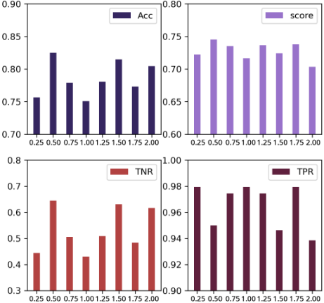
In this section, we evaluate the performance of our model as a function of the weight of contrastive learning loss. We have tested the TPR, TNR, Accuracy and Challenge Score of models trained using different weights of the contrastive loss. Weight starts at 0.25 and ends at 2, with the step of 0.25. As Figure 2 shows, we can see that the model achieves the best score, accuracy and TPR and quite well TNR at the weight of 0.5. Also, we can see that larger weights of contrastive learning loss bring lower TPR, but relatively, there is an increase in TNR. This indicates that a larger contrastive learning loss will improve the model's ability to identify negative samples, but does not have much effect on the recognition ability of the overall model.
| Components | Retrospective | Real-time | |||||||||
|---|---|---|---|---|---|---|---|---|---|---|---|
| Diffusion Model | S-norm | Transformer Encoder | Constractive Learning | TPR | TNR | Score | ACC | TPR | TNR | Score | ACC |
| ✓ ✓ ✓ ✓ | ✓ ✓ ✓ | 97.928 97.442 | 37.025 39.557 52.330 | 69.220 69.206 74.225 68.568 | 72.567 73.338 78.657 | 97.698 97.954 | 37.634 37.993 | 68.980 69.658 | 72.687 72.985 74.179 | ||
| ✓ | ✓ | 97.442 | 52.688 | 74.528 | 77.164 | 97.442 | 41.577 | 70.000 | |||
| ✓ | ✓ | 94.629 | 93.350 | 60.215 | 68.863 | 79.552 | |||||
| ✓ | ✓ | 95.396 | 64.516 | 82.537 | 95.908 | 62.724 | 74.932 | 82.090 | |||
5.3 Interpretability of Model
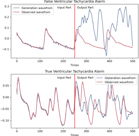
To explain how our model works, we visualized the results of the model on a true ventricular tachycardia waveform and a false ventricular tachycardia waveform. As Figure 3 shows, false ventricular tachycardia alarms are reflected in a flat and regular waveform on the APB channel. This could be due to noise on other channels causing this sample to be classified as a false alarm, when in fact it could be a normal blood pressure waveform. In contrast, true ventricular tachycardia waveforms typically exhibit irregular shapes characterized by high frequency. When the model decisions are false alarms, the generated result of the model is usually a waveform with high frequency with irregularity, which leads to a large difference between the generated and the actual samples. And when the candidate is a true arrhythmia alarm, the distance between the observed and the generated waveform is smaller. Although there are still differences in phase, frequency and amplitude between the generated and the true alarm waveform, have smaller differences compared to the distance between the generated waveform and the false samples.
Figure 3: Results generated by the model on true alarm and false alarm waveforms in the Arterial Blood Pressure (ABP) channel.
6 Conclusions
In this paper, we leverage a generative approach to detect false alarms in ICUs. In order to generate high-quality patients' physiological waveforms, we propose a Conditional Diffusion model based on Contrastive Learning for the generation of waveforms corresponding to real arrhythmias events. During the training process, we use the InfoNCE loss to maximize the distance between positive andnegative sample features to generate better waveforms corresponding to true arrhythmia events. The experimental results on the MIMIC II dataset demonstrate that our model outperforms other models on the ICU false alarm detection task. In addition, our proposed model can potentially be applied to other tasks in time series, such as anomaly detection in time series.
Acknowledgements
This work is in part funded by the NSFC, China under Grants 61902309; in part by the Fundamental Research Funds for the Central Universities, China (xxj022019003); in part by China Postdoctoral Science Foundation (2020M683496); and in part by the National Postdoctoral Innovative Talents Support Program, China (BX20190273); and in part funded by the NIH Grant R01EB030362.
@inproceedings{ijcai2023p546,
  title     = {A Diffusion Model with Contrastive Learning for ICU False Arrhythmia Alarm Reduction},
  author    = {Wu, Feng and Zhao, Guoshuai and Qian, Xueming and Lehman, Li-wei H.},
  booktitle = {Proceedings of the Thirty-Second International Joint Conference on
               Artificial Intelligence, {IJCAI-23}},
  publisher = {International Joint Conferences on Artificial Intelligence Organization},
  editor    = {Edith Elkind},
  pages     = {4912--4920},
  year      = {2023},
  month     = {8},
  note      = {Main Track},
  doi       = {10.24963/ijcai.2023/546},
  url       = {https://doi.org/10.24963/ijcai.2023/546},
}
TY - CPAPER TI - A Diffusion Model with Contrastive Learning for ICU False Arrhythmia Alarm Reduction AU - Wu, Feng AU - Zhao, Guoshuai AU - Qian, Xueming AU - Lehman, Li-wei H. T2 - Proceedings of the Thirty-Second International Joint Conference on Artificial Intelligence, IJCAI-23 PB - International Joint Conferences on Artificial Intelligence Organization PY - 2023 SP - 4912 EP - 4920 DO - 10.24963/ijcai.2023/546 UR - https://doi.org/10.24963/ijcai.2023/546 ER -Copied
Machine-readable versions of this paper, for tools and AI agents:





