
Deep Hashing-based Dynamic Stock Correlation Estimation via Normalizing Flow
Proceedings of the Thirty-Second International Joint Conference on Artificial Intelligence. Main Track. Pages 4993-5001.
https://doi.org/10.24963/ijcai.2023/555
Keywords
- Multidisciplinary Topics and Applications: MDA: Finance
- Machine Learning: ML: Representation learning
Abstract
In financial scenarios, influenced by common factors such as global macroeconomic and sector-specific factors, stocks exhibit varying degrees of correlations with each other, which is essential in risk-averse portfolio allocation. Because the real risk matrix is unobservable, the covariance-based correlation matrix is widely used for constructing diversified stock portfolios. However, studies have seldom focused on dynamic correlation matrix estimation under the non-stationary financial market. Moreover, as the number of stocks in the market grows, existing correlation matrix estimation methods face more serious challenges with regard to efficiency and effectiveness. In this paper, we propose a novel hash-based dynamic correlation forecasting model (HDCF) to estimate dynamic stock correlations. Under structural assumptions on the correlation matrix, HDCF learns the hash representation based on normalizing flows instead of the real-valued representation, which performs extremely efficiently in high-dimensional settings. Experiments show that our proposed model outperforms baselines on portfolio decisions in terms of effectiveness and efficiency.
- [Bickel and Levina, 2008] Peter J Bickel and Elizaveta Lev- ina. Covariance regularization by thresholding. The An- nals of statistics, 36(6):2577-2604, 2008.
- [Bollerslev et al., 1988] Tim Bollerslev, Robert F. Engle, and Jeffrey M. Wooldridge. A capital asset pricing model with time-varying covariances. Journal of Political Economy, 96:116 -131, 1988.
- [Cao et al., 2017] Yue Cao, Mingsheng Long, Jianmin Wang, and Shichen Liu. Deep visual-semantic quantiza- tion for efficient image retrieval. 2017 IEEE Conference on Computer Vision and Pattern Recognition (CVPR), pages 916-925, 2017.
- [Chandrasekaran et al., 2010] Venkat Chandrasekaran, Pablo A. Parrilo, and Alan S. Willsky. Latent variable graphical model selection via convex optimization. 2010 48th Annual Allerton Conference on Communication, Control, and Computing (Allerton), pages 1610-1613, 2010.
- [Chen et al., 2013] Xiaohui Chen, Mengyu Xu, and Wei Biao Wu. Covariance and precision matrix estimation for high-dimensional time series. Annals of Statistics, 41:2994-3021, 2013.
- [Chen et al., 2019] Jia Chen, Degui Li, and Oliver Lin- ton. A new semiparametric estimation approach for large dynamic covariance matrices with multiple conditioning variables. Journal of Econometrics, 212(1):155-176, 2019. Big Data in Dynamic Predictive Econometric Mod- eling.
- [Elton and Gruber, 1973] Edwin J. Elton and Martin J. Gru- ber. Estimating the dependence structure of share prices -implications for portfolio selection. Journal of Finance, 28:1203-1232, 1973.
- [Elton et al., 1978] Edwin J. Elton, Martin J. Gruber, and Thomas J. Urich. Are betas best. Journal of Finance, 33:1375-1384, 1978.
- [Engle et al., 2017] Robert F. Engle, Olivier Ledoit, and Michael Wolf. Large dynamic covariance matrices. Jour- nal of Business & Economic Statistics, 37:363 -375, 2017.
- [Engle, 2002] Robert Engle. Dynamic conditional correla- tion: A simple class of multivariate generalized autore- gressive conditional heteroskedasticity models. Journal of Business & Economic Statistics, 20(3):339-350, 2002.
- [Engle, 2009] Robert Engle. Anticipating Correlations: A New Paradigm for Risk Management. Princeton University Press, 2009.
- [Fama and French, 1989] Eugene F. Fama and Kenneth R. French. Business conditions and expected returns on stocks and bonds. Journal of Financial Economics, 25:23- 49, 1989.
- [Fama and French, 1993] Eugene F. Fama and Kenneth R. French. Common risk factors in the returns on stocks and bonds. Journal of Financial Economics, 33:3-56, 1993.
- [Fan et al., 2007] Jianqing Fan, Yingying Fan, and Jinchi Lv. High dimensional covariance matrix estimation using a factor model. Journal of Econometrics, 147:186-197, 2007.
- [Fan et al., 2013a] Jianqing Fan, Fang Han, and Han Liu. Challenges of big data analysis. National science review, 1 2:293-314, 2013.
- [Fan et al., 2013b] Jianqing Fan, Yuan Liao, and Martina Mincheva. Large Covariance Estimation by Threshold- ing Principal Orthogonal Complements. Journal of the Royal Statistical Society Series B: Statistical Methodol- ogy, 75(4):603-680, 08 2013.
- [Friedman et al., 2008] Jerome H. Friedman, Trevor J. Hastie, and Robert Tibshirani. Sparse inverse covariance estimation with the graphical lasso. Biostatistics, 9 3:432- 41, 2008.
- [Gong et al., 2013] Yunchao Gong, Svetlana Lazebnik, Al- bert Gordo, and Florent Perronnin. Iterative quantization: A procrustean approach to learning binary codes for large- scale image retrieval. IEEE Transactions on Pattern Anal- ysis and Machine Intelligence, 35:2916-2929, 2013.
- [Jiang and Li, 2016] Qing-Yuan Jiang and Wu-Jun Li. Deep cross-modal hashing. 2017 IEEE Conference on Computer Vision and Pattern Recognition (CVPR), pages 3270- 3278, 2016.
- [Jordan et al., 1999] Michael I. Jordan, Zoubin Ghahramani, T. Jaakkola, and Lawrence K. Saul. An introduction to variational methods for graphical models. Machine Learn- ing, 37:183-233, 1999.
- [Ke et al., 2020] Yuan Ke, Heng Lian, and Wenyang Zhang. High-dimensional dynamic covariance matrices with ho- mogeneous structure. Journal of Business & Economic Statistics, 40:96 -110, 2020.
- [Kingma and Ba, 2014] Diederik P. Kingma and Jimmy Ba. Adam: A method for stochastic optimization. CoRR, abs/1412.6980:1-15, 2014.
- [Lan et al., 2017] Shiwei Lan, Andrew J. Holbrook, Gabriel A. Elias, Norbert J. Fortin, Hernando C. Ombao, and Babak Shahbaba. Flexible bayesian dynamic mod- eling of correlation and covariance matrices. Bayesian analysis, 15 4:1199-1228, 2017.
- [Liang et al., 2021] Qianqiao Liang, Mengying Zhu, Xi- aolin Zheng, and Yan Wang. An adaptive news-driven method for cvar-sensitive online portfolio selection in non- stationary financial markets. In Zhi-Hua Zhou, editor, Pro- ceedings of the Thirtieth International Joint Conference on Artificial Intelligence, IJCAI-21, pages 2708-2715. Inter- national Joint Conferences on Artificial Intelligence Orga- nization, 8 2021. Main Track.
- [Liu et al., 2017] X. Liu, Lili Zhao, Dajun Ding, and Yajiao Dong. Deep hashing with category mask for fast video retrieval. ArXiv, abs/1712.08315, 2017.
- [Markowitz, 1952] Harry Markowitz. Harry m. markowitz. Portfolio selection, Journal of Finance, 7(1):77-91, 1952.
- [Rangel and Engle, 2012] José Gonzalo Rangel and Robert F Engle. The factor-spline-garch model for high and low frequency correlations. Journal of Business & Economic Statistics, 30(1):109-124, 2012.
- [Sak et al., 2014] Hasim Sak, Andrew W. Senior, and Franc ¸oise Beaufays. Long short-term memory based re- current neural network architectures for large vocabulary speech recognition. ArXiv, abs/1402.1128:1-5, 2014.
- [Shen and Wang, 2017] Weiwei Shen and Jun Wang. Portfo- lio selection via subset resampling. In Proceedings of the Thirty-First AAAI Conference on Artificial Intelligence, AAAI'17, page 1517-1523. AAAI Press, 2017.
- [Xia et al., 2014] Rongkai Xia, Yan Pan, Hanjiang Lai, Cong Liu, and Shuicheng Yan. Supervised hashing for image re- trieval via image representation learning. In Proceedings of the Twenty-Eighth AAAI Conference on Artificial Intel- ligence, AAAI'14, page 2156-2162. AAAI Press, 2014.
- [Yang et al., 2017] Erkun Yang, Cheng Deng, Wei Liu, Xi- anglong Liu, Dacheng Tao, and Xinbo Gao. Pairwise re- lationship guided deep hashing for cross-modal retrieval. AAAI'17, page 1618-1625. AAAI Press, 2017.
- [Yuan et al., 2019] Li Yuan, Tao Wang, Xiaopeng Zhang, Francis E. H. Tay, Zequn Jie, Wei Liu, and Jiashi Feng. Central similarity quantization for efficient image and video retrieval. 2020 IEEE/CVF Conference on Computer Vision and Pattern Recognition (CVPR), pages 3080- 3089, 2019.
- [Zhu et al., 2016] Han Zhu, Mingsheng Long, Jianmin Wang, and Yue Cao. Deep hashing network for efficient similarity retrieval. AAAI'16, page 2415-2421. AAAI Press, 2016.
- [Zhu et al., 2020] Mengying Zhu, Xiaolin Zheng, Yan Wang, Qianqiao Liang, and Wenfang Zhang. Online portfolio selection with cardinality constraint and trans- action costs based on contextual bandit. In Christian Bessiere, editor, Proceedings of the Twenty-Ninth Interna- tional Joint Conference on Artificial Intelligence, IJCAI- 20, pages 4682-4689. International Joint Conferences on Artificial Intelligence Organization, 7 2020. Special Track on AI in FinTech. IJCAI
- [Zhu et al., 2022] Haoren Zhu, Shih-Yang Liu, Pengfei Zhao, Yingying Chen, and Dik Lun Lee. Forecasting asset dependencies to reduce portfolio risk. 36:4397-4404, Jun. 2022.
References were extracted automatically from the PDF and may contain errors.
Full text extracted automatically from the PDF; figures, tables and equations may differ. The PDF is the version of record.
1 Introduction
In financial scenarios, influenced by common factors such as global macroeconomic and sector-specific factors [Fama and French, 1989; Fama and French, 1993], stocks exhibit varying degrees of correlations with each other. For instance, stocks sharing the same industry risks tend to have highly correlated returns. These correlations between stocks play a central role in risk-averse portfolio allocation. According to Markowitz's theory [Markowitz, 1952], portfolio optimization heavily relies on the correlations between the returns of different stocks to diversify risk. In risk-averse portfolio allocation, a covariance-based correlation matrix, i.e., correlation coefficients matrix of stocks, can directly reflect such correlations in a risk perspective, which is widely used for constructing diversified stock portfolios [Fan et al., 2013a; Ke et al., 2020].
∗Corresponding Author
There is a large body of work on covariance-based correlation matrix estimation, which can be divided into two categories: static and dynamic methods. Static estimation methods, like POET [Fan et al., 2013b], often cap-
ics of these correlations. Alternatively, there is impressive literature on dynamic estimation techniques, such as parametric GARCH-based methods [Bollerslev et al., 1988; Engle et al., 2017; Lan et al., 2017; Ke et al., 2020] and non-/semi-parametric kernel approaches [Chen et al., 2013; Chen et al., 2019]. However, the above estimation methods face a challenging problem when markets include a large variety of stocks, i.e., the limited sample size problem in highdimensional settings. This problem especially becomes more severe for dynamic correlation matrix estimation. The reason is twofold. Firstly, obtaining adequate data samples in nonstationary markets is challenging due to the limited utility of too old data in reflecting the present dynamic changes in correlation. Secondly, there are more parameters to estimate in the time-varying estimation model. To address this problem, researchers have made several structural assumptions on correlation matrices; the two most common ones are low-rank factor models [Fama and French, 1989; Fan et al., 2007] and (conditional) sparsity [Bickel and Levina, 2008; Friedman et al., 2008] (or a combination of both [Fan et al., 2013b; Chandrasekaran et al., 2010]). Inspired by earlier work on the structural assumptions, we creatively propose an end-toend dynamic correlation matrix forecasting method between different stocks, aiming to enhance the efficiency of correlation matrix forecasting in portfolio diversification.
Due to the excellent efficiency in storage and computation, deep hashing yields breakthrough results in image retrieval [Cao et al., 2017; Xia et al., 2014; Gong et al., 2013], video retrieval [Liu et al., 2017; Yuan et al., 2019], and cross-modal retrieval [Jiang and Li, 2016; Yang et al., 2017]. Deep hashing methods have a good ability to learn complex hash functions and obtain high-quality hash representations using the powerful representation capabilities of deep learning. Based on the aforementioned analysis, we design a hashbased dynamic correlation matrix forecasting model (HDCF). HDCF learns the binary representation of the correlation matrix, which performs the dynamic correlation matrix forecasting and portfolio risk reduction task extremely efficiently.
However, it is non-trivial to model a hash-based correlation matrix prediction model, where the challenge is twofold.
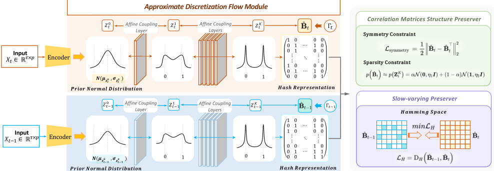
Firstly, CH1: How to implement optimization on discrete hash representations? Due to the discrete property of the binary hash representations, the optimization is an intractable problem and is prone to the vanishing gradient problem. To address CH1, HDCF contains an approximate discretization flow module (ADFM). A series of reversible transformations based on normalizing flow are performed on a real-valued representation that follows a priori normal distribution to generate an approximate binary representation. Then, the hash representation is generated by the binarization operations. Finally, we directly optimize the hash representation based on the approximate binary representation.
Secondly, CH2: How to preserve the properties of the correlation matrix? On the one hand, considering that the correlation matrix is dynamically changing, from a practical point of view, the difference between the correlation matrices in two successive periods should not be too large, i.e., the evolution pattern of the correlation matrix is slowvarying. On the other hand, the correlation matrix has symmetry. To tackle CH2, we design two structure preserving components, i.e., slow-varying preserver (SVP) and correlation matrix structure preserver (CMSP). SVP constructs pairwise metric learning of hash representations in two successive periods in Hamming space. In CMSP, we design two regularizers to impose structural constraints on the correlation matrix, which is fast and flexible.
To the best of our knowledge, this is the first work in the literature on end-to-end deep hashing-based correlation matrix estimation in portfolio diversification. Our main contributions are as follows:
- We propose a novel deep hashing model called HDCF, which focuses on efficient dynamic correlation matrix estimation for a risk-averse portfolio allocation;
- In HDCF, we design three special modules, i.e., ADFM, SVP, and CMSP, to address the two challenges. Specifically, ADFM applies normalizing flow to learn the binary representation of the dynamic correlation matrix (for addressing CH1), and two structure preserving components (SVP and CMSP) construct three constraints based on regularizers and pair-wise metric learning to preserve the properties of the correlation matrix (for addressing CH2).
- We have conducted extensive experiments on three realworld datasets to demonstrate HDCF's superiority over the state-of-the-art covariance-based correlation matrix estimation methods. The results highlight HDCF is not only effective for the portfolio decision task but also efficient in large-scale scenarios.
2 RelatedWork
2.1 Risk-averse Portfolio Selection
Since the seminal work of Markowitz [Markowitz, 1952], the mean-variance paradigm has been at the heart of the modern portfolio theory, which is the theoretical cornerstone of the risk-averse portfolio selection problem. In risk-averse portfolios, correlations between stocks are an important consideration, where lower stock correlations imply a higher diversification in the portfolio, which can diversify risk effectively. As stock correlations change over time, a risk-averse portfolio in one step may no longer be diversified in the next step and may incur unexpected losses [Engle, 2009]. Therefore, we need to model the dynamic correlation matrix in order to achieve a consistent low-risk level in a portfolio.
2.2 Dynamic CorrelationMatrix Prediction Methods
Multivariate GARCH (MGARCH) is a class of models that can estimate time-varying stock correlations. The Dynamic Conditional Correlation (DCC) model [Engle, 2002] and its variants [Engle et al., 2017; Rangel and Engle, 2012] address the dynamic structure of stock correlations by parameterizing conditional correlations. However, these statistically oriented methods (1) hold unrealistic statistical assumptions that make them unsuitable for real data and (2) use linear regression in parameter estimation, which is challenging to model correlations in large-scale settings. Compared with existing works, on the one hand, our framework is based on deep hashing to learn binary correlation representation, which makes our model extremely efficient even when the number of stocks grows substantially. On the other hand, using regularizers to make structural constraints on the dynamic correlation matrix is flexible.
3 Preliminaries and ProblemFormulation
Preliminaries. In the financial market, given the historical daily prices of stock i: {pi0 , pi1 , . . . , piT }, where pit denotes the price of stock i at time t, the price relative of stock i at time t is calculated by:
Let ft (si, sj) denote the correlation measurement between stock i and stock j at time t. For correlation function f of two stocks si and sj in period [t-∆, t], ft(si, sj) is calculated as follows:
It is natural to use matrix group all pair-wise correlations, then the correlation matrix at time t can be denoted as Γt, formulated as:
When the computation of correlation coefficient is used as the measure function ft, Γt is called a covariance-based correlation matrix.
Definition 1 (Covariance-based Correlation Matrix). Covariance-based correlation matrix of stocks is a symmetric matrix composed of the correlation coefficients of a group of stocks. We can calculate the predicted covariance matrix ˆΣt at round t:
where ˆΓt denotes the covariance-based correlation matrix predicted by the estimation method, s denotes the standard deviation vector at round t, and diag(s) is to create a diagonal matrix with s.
Problem Formulation. We consider a portfolio diversification problem with p stocks during T trading rounds. We start by setting up notation. At each trading round t, the price relatives of the stocks are denoted by a vector rt = (r1 t , r2 t , . . . , rp t ). The price relative ri t is bounded in a closed interval [C1,C2] (C1 and C2 are constants satisfying 0 < C1 ≤ C2). The portfolio diversification problem at round t is to determine an optimal portfolio πt based on the correlations between all the p stocks at round t. The portfolio πt is defined by a weight vector wt = (w1 t , w2 t , . . . , wp t ) satisfying the constraint that every wi t is non-negative and the sum of all wt equals to one, i.e., w ∈ ∆p = {w | 0 ≤ w ≤ 1, w⊤1 = 1}, where wi t indicates the proportion of wealth allocated to the stock i. The goal is to forecast dynamic correlation matrix Γt at round t based on the multivariate time series {rt-τ:t-1} (for simplicity called Xt) up to round t - 1. τ is the window size on price-relative sequences.
Definition 2 (Minimum-variance Portfolio). A minimumvariance portfolio wt at round t is constructed as follows:
where Eq.(5) is an objective function according to the meanvariance portfolio criterion [Markowitz, 1952], Σt is the portfolio's risk matrix, µt is the mean vector of stock price relatives, and E is the expected portfolio's return decided by the investor.
4 Method
4.1 Overview of HDCF
The architecture of our proposed HDCF is presented in Figure 1, which includes three key modules, i.e., approximate discretization flow module (ADFM), slow-varying preserver (SVP), and correlation matrices structure preserver (CMSP). Details of each module are as follows:
- ADFM uses a recurrent neural network (RNN), here an LSTM [Sak et al., 2014], to model correlations between stocks as real-valued representations that obey prior normal distribution. Normalizing flow is subsequently deployed to achieve pre-hash representation that obeys a continuous but approximately discrete distribution. Finally, the binarization operation on this distribution is recruited to output the hash representation of the correlation matrix (§4.2).
- SVP supposes to learn hash representations between two successive periods supervised by the similarity under the slow-varying assumption. The pair-wise similarity would encourage hash correlation matrices of successive periods to be close to each other. Through such pair-wise similarity learning, the similarity information between correlation matrix pairs can be preserved, yielding highquality hash correlation matrices (§4.3).
- CMSP utilizes the properties of symmetry matrix and sparse matrix to learn binary correlation matrices with the correct structure, improving the hash representation of correlation matrix (§4.4).
4.2 Approximate Discretization FlowModule (ADFM)
Modeling. For the stock correlation forecasting task at round t, the objective we seek to maximize is the likelihood of the correlation matrix Γt, i.e., p(Γt). Formally, we determine the likelihood p(Γt) in Eq.(6) by introducing the predicted hash representation ˆBt of the correlation matrix at round t as the condition:
We assume any correlation coefficient γ (i,j) t in Γt is Gaussian distributed around their true mean, and ˆb(i,j) t is the bit of ˆBt at the corresponding position, such that we can compute the conditional log-likelihood as follows:
where the variance σ2 γ is constant, thus providing an equal weighting of correlation coefficients.
However, the exact value of the variance is irrelevant since maximizing Eq.(7) corresponds to simply minimizing the squared error (MSE) of the mean term, i.e., γ (i,j) t - ˆb(i,j) t . The conditional log-likelihood within the expectation term in Eq.(6) can be considered a reconstruction term, which represents how well the observed correlation matrix Γt can be decoded from the hash representations ˆBt. Thus, we define the reconstruction error loss function as follows:
Furthermore, maximization in Eq.(6) is still intractable. Thus we need to introduce variational inference [Jordan et al., 1999]. Variational inference devotes to approximate posterior qϕ ( ˆBt | Xt) to surrogate the true intractable posterior p ( ˆBt), where ϕ denotes parameters on neural networks. Formally, variational inference in this work seeks to simultaneously minimize the Kullback-Leibler divergence KL (qϕ ( ˆBt | Xt) ∥p ( ˆBt)) to achieve the optimal ϕ. During the learning process with the above variational inference, an Evidence Lower BOund can be drawn in Eq.(9). Therefore, we can use ELBO maximization as a proxy to indirectly maximize the log-likelihood function, as follows:
where the second term in ELBO is a regularizer that constrains the form of the approximate posterior.
Calculation. Firstly, we adopt LSTM to encode the stocks' historical returns Xt to obtain a latent state ht that represents the concatenation of the LSTM cell state vectors and the LSTM-unit output vectors at time t, i.e., ht = gθ (Xt, ht-1), where g refers to the hidden-state evolution at each timestep and the subscript θ indicates model parameters.
Secondly, we use a linear layer to generate the mean and variance of the base distribution qθ (z0,(i,j) ) as follows:
where z0,(i,j) t is the latent random variable sampled from qθ (z0,(i,j) t ), and z0,(i,j) t with ∀i, j ∈ {0, ..., p -1} forms the real-valued representation Z0t ∈ Rp×p .
Then due to ˆBt's discrete property, HDCF transforms the base distribution by stacking K affine coupling transformation layers, and the output of the Kth affine coupling transformation layer is ZKt ∈ Rp×p . Since every transformation in normalizing flow is invertible: Using the change-of-variables formula, we can write the log-likelihood of qϕ (ZKt ) as used in likelihood maximization, as follows:
where ϕ denotes model parameters, and qN is the probability density function of the p2 -dimensional normal distribution, and ∂Zl+1 t ∂Zlt is the Jacobian matrix of the transformation Zlt→Zl+1 t on the lth affine coupling layer.
Finally, we achieve the hash representation ˆBt of the correlation matrix at round t, where
is applied element-wisely, and zK,(i,j) t is the element in ZKt .
Meanwhile, we prefer that the hash representation ˆBt conforms to the Bernoulli distribution. However, the Bernoulli distribution is discrete, which makes it much more difficult to be optimized. Therefore, to control the quantization error between Γt and ˆBt to learn high-quality hash representations, we use MSE between Γt and ZKt to approximate Eq.(8) as
Moreover, to approximate the Bernoulli distribution, we utilize the approximate mixture multivariate normal distribution defined as
where ηI denotes the covariance matrix of the corresponding normal distribution. Here, η is set to 0.005 in our experiments. Therefore the KL term in Eq.(9) can be written by:
Finally, the loss function for the optimal hash representations can be defined as:
It is worth noting that ˆBt ∈ {0, 1}p×p , so we scale the value range of the real correlation matrix Γt to [0, 1] through a reversible linear transformation for better supervision.
4.3 Slow-varying Preserver (SVP)
Considering that the correlation matrix is dynamic, we assume the evolving pattern of the stock correlation matrix is slow-varying. Thus, predicted binary correlation matrices of round t and round t -1, ˆBt and ˆBt-1, are encouraged to be close to each other in the Hamming space. Therefore, we design a loss function for the slow-varying pattern as follows:
where DH (·, ·) denotes the Hamming distance between two binary matrices. Here we use the squared L2-norm to measure the distance between the approximate real-valued representations to replace the Hamming distance.
4.4 CorrelationMatrices Structure Preserver (CMSP)
To further enhance the quality of the hash representation, in CMSP we design two regularizers to preserve the properties of the correlation matrix. First, the correlation matrix is symmetric, i.e., ˆBt = ˆB⊤t , where ˆB⊤t is the transpose of ˆBt. Thus, we design a loss function to constrain the distance between ˆBt and ˆB⊤t :
Based on the sparsity assumption of the covariance-based correlation matrix, we redefine Eq.(15) as:
where we add the sparsity control coefficient α, the larger the α, the sparser ˆBt is. α needs to be manually specified as needed. With the sparsity control, the hash representation loss function in Eq.(17) is represented as LΓ(α).
4.5 Combined Loss Function
Next, we arrive at the fused loss function combining the three
Supposed that there are N rounds of data {Xt | t = 1, ...,N} being trained, and our goal is to minimize the overall loss function:
where ˆBt ∈ {0, 1}p×p is the predicted hash correlation matrix at round t with t ∈ {1, . . . , N} and Γt ∈ Rp×p is the real covariance-based correlation matrix at round t. Z0t ∈ Rp×p is the real-valued representation under the base distribution. Zlt ∈ Rp×p is the output of the lth affine coupling transformation layer, l ∈ {1, . . . ,K}, and zK,(i,j) t refers to elements in ZKt . With this objective function, the network is trained using back-propagation algorithm with the mini-batch stochastic gradient descent (SGD) method.
5 Experiments
In this section, we aim to answer the following questions through empirical studies: Q1: How does HDCF perform on cumulative return over the trading rounds? Q2: How does HDCF perform in reducing risk? Q3: How can SVP and CMSP contribute to the performance of HDCF? Q4: How does the hash-based correlation prediction model perform on computational efficiency?
5.1 Experimental Settings
Dataset Descriptions. Experiments are conducted on three representative datasets, i.e., SP500 N, SP500 O, and HS300 datasets 1 . SP500 N is a newly collected U.S. market dataset containing the SP500 index constituent stocks, which covers the volatile COVID-19 period. SP500 O is a widely used dataset also containing the SP500 index constituent stocks, which covers the well-known 2007 - 2008 financial crisis period. HS300 is a newly collected dataset containing the CSI300 index constituent stocks in China, which covers the COVID-19 period. Some newly listed constituent stocks with excessive missing data have been eliminated. All datasets are divided into non-overlapping training/validation/test sets, as described in Table 1.
Baselines. Six baselines are classified into three groups, and two versions of our proposed approaches are compared: (1) Static/Dynamic Correlation Matrix Estimation Methods: Full Historical Model (FHM) [Elton et al., 1978] is the simplest method to adopt the past correlation value as the future correlation coefficient. Constant Correlation Model (CCM) [Elton and Gruber, 1973; Elton et al., 1978] estimates the correlation of each pair of stocks to be the average correlation of all pairs of stocks in a given portfolio. Dynamic Conditional Correlation GARCH (DCC-GARCH) [Engle, 2002] is a multivariate time-series-based method that considers the dynamic property of correlation in the model by parameterizing the conditional correlations to forecast the future correlation matrix.
- Sparse Correlation Matrix Estimation Methods: Hard Thresholding [Bickel and Levina, 2008] and Graphical Lasso [Friedman et al., 2008] are multivariate time-seriesbased methods that consider regularizing the correlation matrix by hard thresholding and lasso penalty, respectively, under the assumption of sparsity.
- Deep Learning Model For Correlation Matrix Prediction: ADNN [Zhu et al., 2022] is the state-of-the-art deep learning model for correlation matrix prediction and portfolio risk reduction.
(4) Simplified versions of HDCF: HDCF-flow is HDCF without structure preserver SVP and CMSP, which means that the predicted binary correlation matrix cannot guarantee symmetry and a slow-varying pattern. HDCF-hash is HDCF without SVP, CMSP, and ADFM, which is a general deephashing method with LSTM as encoder and bi-modal Laplacian prior [Zhu et al., 2016] for quantization.
1 Data is collected from https://finance.yahoo.com/, https://www. kaggle.com/camnugent/sandp500, and https://tushare.pro/, respectively.
| Dataset | # Stock | Training Data Range | Validation Data Range | Test Data Range |
|---|---|---|---|---|
| SP500 N | 511 | 01/01/2020 - 12/31/2020 | 01/01/2021 - 06/30/2021 | 07/01/2021 - 06/30/2022 |
| SP500 O | 478 | 10/18/2006 - 06/30/2007 | 07/01/2007 - 12/31/2007 | 01/01/2008 - 11/20/2013 |
| HS300 | 272 | 01/02/2020 - 12/31/2020 | 01/01/2021 - 06/30/2021 | 07/01/2021 - 06/30/2022 |
| SP500 N | SP500 O | HS300 | |||||
|---|---|---|---|---|---|---|---|
| Categories | Baselines | CW | APY | CW | APY | CW | APY |
| Market | Index 2 | 0.89 | -0.11 | 1.22 | 0.03 | 0.86 | -0.15 |
| Static/Dynamic Estimation Methods | FHM CCM DCC-GARCH | 0.63 0.68 0.59 | -0.37 -0.32 -0.41 | 0.21 0.91 0.12 | -0.23 -0.02 -0.30 | 0.63 0.55 0.58 | -0.38 -0.47 -0.43 |
| Sparse Correlation Matrix Estimation Methods | Hard Thresholding Graphical Lasso | 0.61 0.84 | -0.39 -0.16 | 0.15 1.04 | -0.28 0.01 | 0.79 0.75 | -0.22 -0.26 |
| Deep Prediction Model | ADNN | 0.86 ± 0.024 | -0.14 ± 0.024 | 1.68 ± 0.465 | 0.09 ± 0.054 | 0.92 ± 0.004 | -0.08 ± 0.004 |
| HDCF (Our) | HDCF HDCF-flow HDCF-hash | 0.87 ± 0.003 0.87 ± 0.004 0.86 ± 0.005 | -0.13 ± 0.003 -0.13 ± 0.004 -0.14 ± 0.005 | 1.99 ± 0.015 1.84 ± 0.036 1.78 ± 0.022 | 0.12 ± 0.001 0.12 ± 0.038 0.10 ± 0.002 | 0.91 ± 0.019 0.89 ± 0.003 0.87 ± 0.004 | -0.09 ± 0.019 -0.11 ± 0.001 -0.13 ± 0.005 |
| Improvement 3 p-value 4 | 1.16% 0.000 | 7.14% 0.000 | 18.45% 0.000 | 33.33% 0.000 | -1.09% 0.000 | -12.50% 0.002 | |
| SP500 N | SP500 O | HS300 | |||||
| Categories | Baselines | MD | AVO | MD | AVO | MD | AVO |
| Market | Index | 0.24 | 0.25 | 0.54 | 0.20 | 0.28 | 0.20 |
| Static/Dynamic Estimation Methods | FHM CCM DCC-GARCH | 0.39 0.34 0.42 | 0.16 0.17 0.15 | 0.81 0.29 0.88 | 0.20 0.16 0.18 | 0.43 0.46 0.46 | 0.21 0.18 0.20 |
| Sparse Correlation Matrix Estimation Methods | Hard Thresholding Graphical Lasso | 0.41 0.23 | 0.16 0.20 | 0.85 0.25 | 0.19 0.27 | 0.33 0.28 | 0.19 0.21 |
| Deep Prediction Model | ADNN | 0.23 ± 0.017 | 0.22 ± 0.012 | 0.38 ± 0.150 | 0.15 ± 0.075 | 0.27 ± 0.006 | 0.13 ± 0.008 |
| HDCF (Our) | HDCF HDCF-flow HDCF-hash | 0.22 ± 0.002 0.22 ± 0.003 0.23 ± 0.004 | 0.19 ± 0.001 0.19 ± 0.000 0.20 ± 0.000 | 0.22 ± 0.007 0.23 ± 0.016 0.26 ± 0.004 | 0.25 ± 0.0000 0.25 ± 0.001 0.26 ± 0.000 | 0.28 ± 0.002 0.28 ± 0.007 0.30 ± 0.002 | 0.19 ± 0.000 0.20 ± 0.001 0.20 ± 0.002 |
| Improvement p-value | 4.35% 0.000 | -26.67% 0.000 | 12.00% 0.000 | -66.67% 0.001 | -3.70% 0.000 | -46.15% 0.000 | |
Implementation details. We implement all experiments using PyTorch and conduct the experiments on an NVIDIA RTX 3090 GPU. We tune the hyper-parameters of HDCF and baseline models to their best values for a fair comparison. We adopt Adam [Kingma and Ba, 2014] as the optimizer for training. We set window size as 7, batch size as 16, and learning rate as 1e - 6. The number of affine coupling layers is set as 10. We set the sparsity control coefficient α = 0.6, 0.6, and 0.3 on SP500 N, SP500 O, and HS300, respectively. The expected return E in portfolio construction is set as 0.
Metrics. We use four standard metrics to measure portfolios' performance, which are widely used in portfolio tasks [Liang et al., 2021; Shen and Wang, 2017; Zhu et al., 2020].
2 The index is S&P 500 (ˆGSPC) in SP500 O and SP500 N datasets, and CSI 300 (000300.SH) in HS300.
3 Improvement of HDCF over the best-performing baselines.
4 The improvement over the best-performing baselines is significant based on paired t-test at the significance level of 0.05 (p-value with paired t-test).
Cumulative wealth (CW) and Annualized Percentage Yield (APY) measure the portfolios' returns. Maximum drawdown (MD) and Annualized Volatility (AVO) measure the portfolios' drawdown and volatility risks. Generally speaking, higher CW and APY indicate better performance; lower MD and AVO indicate better performance.
The calculation formulas of all four metrics are as follows:
(1) Cumulative wealth (CW) is the total returns yielded
- from a portfolio strategy: CWT = ∏Ti=1 (1 + ri), where ri is the net return at round t.
(2) Annualized Percentage Yield (APY) measures the average wealth increment that one portfolio strategy could achieve compounded in a year, which is defined as APYT = y√CWT - 1, where y is the number of years corresponding to T trading rounds.
(3) Maximum Drawdown (MD) measures the decline from a historical peak in the cumulative wealth, which is defined as MDT = maxt∈(0,T )[max[0, maxi∈(0,t) CWi - CWt]].
(4) Annualized Volatility (AVO) is the annualized standard
deviation of daily returns and multiplied by √AT, where AT is the average trading rounds of annual trading days and AT = 252 for all three datasets.
5.2 Performance on Return
To answer question Q1, we present the CW and APY values achieved by HDCF and the six comparison methods in Table 2. Firstly, HDCF achieves the highest CW value and APY value in SP500 N with average improvements of 1.16% and 7.14%, respectively, over the best-performing comparison methods, and in SP500 O with average improvements of 18.45% and 33.33%. Compared with the deep learning model ADNN, a real-value correlation matrix prediction model using the large length of historical returns (in the paper: 230 days) as input, HDCF utilizes returns only in the past seven days to forecast the binary correlation matrix. With a smaller overhead, the difference between all metrics values in HS300 is no more than 0.01.
Compared with baselines in three groups respectively, we can get the following three conclusions. Firstly, compared with static methods, HDCF models the dynamics of correlations and thus can adapt to ever-changing markets. Compared with dynamic methods without deep learning, HDCF can learn richer features to make predictions accurate enough for asset management. Secondly, HDCF outperforms estimation methods under sparsity assumption because it is difficult to find a suitable threshold value in these approaches to constrain the sparsity of the correlation matrix, and a tiny estimation error can significantly worsen the prediction results. Thirdly, on SP500 N with 511 stocks and SP500 O with 478 stocks, HDCF is superior to ADNN, even when the historical window size is small, which demonstrates that our structural assumptions can fully utilize the limited samples in high-dimensional settings to achieve better accuracy.
5.3 Performance on Risk
To answer Q2, we present the risk (MD) and annualized volatility (AVO) achieved by HDCF and the six comparison methods in Table 2. In terms of risk, i.e., estimating AVO and MD, HDCF outperforms most static/dynamic and sparse correlation matrix estimation methods. In SP500 N and HS300, most of the metric values in HDCF differ no more than 0.1 from ADNN. It is worth noting that HDCF achieves minor standard deviations in all three datasets, demonstrating that our model is robust.
5.4 Ablation Study
Since our predicted correlation matrix is a binary hash representation, we compare HDCF with two hash-based ablation methods: HDCF-hash and HDCF-flow. The experimental results for the ablation study are shown in Table 2, in which HDCF achieves the best performance on CW, APY, MD, and AVO compared with the other two methods, with average improvements of 4.66%, 12.68%, 5.12%, and 3.14%, respectively. On the one hand, compared with HDCF-flow, improvement in structural preservation mechanism can get highquality hash representation for the correlation matrix. On the other hand, compared with the relaxation method of HDCFhash to control the quantization error, normalizing flows can obtain hash representation closer to the real-valued representation and more easily optimized.
5.5 Computation Efficiency
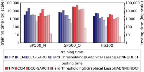
Recall that one of the primary motivations of our proposal is to recruit hash representation for more efficiency, which is essential in large covariance-based correlation matrix prediction. This section examines the efficiency of the correlation matrix prediction by HDCF and six baselines on three datasets SP500 N, SP500 O, and HS300. We record runtimes for all methods in the training and testing phases, i.e., training times and testing times. Note that for deep learning models, the training time refers to the runtime over several epochs to train the model until convergence on the training dataset, and the testing time refers to the runtime to test on the test set.
As is illustrated in Figure 2, HDCF is significantly faster than the six comparison methods and maintains high efficiency consistently across the three datasets with varying numbers of stocks, achieving an average speed improvement factor of 18 in training time and 392 in testing time. This observation demonstrates the efficiency benefit of the hashbased correlation prediction model for high-dimensional scenarios.
6 Conclusions and FutureWork
In this paper, we propose a novel dynamic correlation matrix forecasting method named HDCF to estimate dynamic stock correlations and reduce portfolio risk. HDCF is a deep hashing-based model incorporating normalizing flows to obtain high-quality hash representations and facilitate regularizers to impose structural constraints. Empirical studies demonstrate HDCF is not only effective for the portfolio decision task but also efficient in small-sample and highdimensional settings. For future work, we will study how to incorporate side information, e.g., stock graphs, news, and social media, to model stocks' dynamic correlations in portfolio selection.
Acknowledgments
This work was supported in part by the National Key R&D Program of China (No. 2022YFF0902704) and the "Ten Thousand Talents Program" of Zhejiang Province for Leading Experts (No. 2021R52001).
@inproceedings{ijcai2023p555,
  title     = {Deep Hashing-based Dynamic Stock Correlation Estimation via Normalizing Flow},
  author    = {Zheng, Xiaolin and Liu, Mengpu and Zhu, Mengying},
  booktitle = {Proceedings of the Thirty-Second International Joint Conference on
               Artificial Intelligence, {IJCAI-23}},
  publisher = {International Joint Conferences on Artificial Intelligence Organization},
  editor    = {Edith Elkind},
  pages     = {4993--5001},
  year      = {2023},
  month     = {8},
  note      = {Main Track},
  doi       = {10.24963/ijcai.2023/555},
  url       = {https://doi.org/10.24963/ijcai.2023/555},
}
TY - CPAPER TI - Deep Hashing-based Dynamic Stock Correlation Estimation via Normalizing Flow AU - Zheng, Xiaolin AU - Liu, Mengpu AU - Zhu, Mengying T2 - Proceedings of the Thirty-Second International Joint Conference on Artificial Intelligence, IJCAI-23 PB - International Joint Conferences on Artificial Intelligence Organization PY - 2023 SP - 4993 EP - 5001 DO - 10.24963/ijcai.2023/555 UR - https://doi.org/10.24963/ijcai.2023/555 ER -Copied
Machine-readable versions of this paper, for tools and AI agents:





