
Complex Contagion Influence Maximization: A Reinforcement Learning Approach
Proceedings of the Thirty-Second International Joint Conference on Artificial Intelligence. Main Track. Pages 5531-5540.
https://doi.org/10.24963/ijcai.2023/614
Keywords
- Machine Learning: ML: Reinforcement learning
- Multidisciplinary Topics and Applications: MDA: Web and social networks
- Search: S: Combinatorial search and optimisation
Abstract
In influence maximization (IM), the goal is to find a set of seed nodes in a social network that maximizes the influence spread. While most IM problems focus on classical influence cascades (e.g., Independent Cascade and Linear Threshold) which assume individual influence cascade probability is independent of the number of neighbors, recent studies by sociologists show that many influence cascades follow a pattern called complex contagion (CC), where influence cascade probability is much higher when more neighbors are influenced. Nonetheless, there are very limited studies for complex contagion influence maximization (CCIM) problems. This is partly because CC is non-submodular, the solution of which has been an open challenge.
In this study, we propose the first reinforcement learning (RL) approach to CCIM. We find that a key obstacle in applying existing RL approaches to CCIM is the reward sparseness issue, which comes from two distinct sources. We then design a new RL algorithm that uses the CCIM problem structure to address the issue. Empirical results show that our approach achieves the state-of-the-art performance on 9 real-world networks.
- [Ali et al., 2018] Khurshed Ali, Chih-Yu Wang, and Yi-Shin Chen. Boosting reinforcement learning in competitive influence maxi- mization with transfer learning. In WI, pages 395-400, 2018.
- [Angell and Schoenebeck, 2017] Rico Angell and Grant Schoenebeck. Don't be greedy: Leveraging community structure to find high quality seed sets for influence maximization. In WINE, pages 16-29. Springer, 2017.
- [Backstrom et al., 2006] Lars Backstrom, Dan Huttenlocher, Jon Kleinberg, and Xiangyang Lan. Group formation in large social networks: Membership, growth, and evolution. In KDD, pages 44-54, 2006.
- [Banerjee et al., 2013] Abhijit Banerjee, Arun G Chandrasekhar, Es- ther Duflo, and Matthew O Jackson. The diffusion of microfinance. Science, 341(6144), 2013.
- [Beaman et al., 2021] Lori Beaman, Ariel BenYishay, Jeremy Ma- gruder, and Ahmed Mushfiq Mobarak. Can network theory-based targeting increase technology adoption? American Economic Review, 111(6):1918-43, 2021.
- [Bello et al., 2016] Irwan Bello, Hieu Pham, Quoc V Le, Mo- hammad Norouzi, and Samy Bengio. Neural combinato- rial optimization with reinforcement learning. arXiv preprint arXiv:1611.09940, 2016.
- [Bengio et al., 2021] Yoshua Bengio, Andrea Lodi, and Antoine Prouvost. Machine learning for combinatorial optimization: A methodological tour d'horizon. European Journal of Operational Research, 290(2):405-421, 2021.
- [Borgs et al., 2014] Christian Borgs, Michael Brautbar, Jennifer Chayes, and Brendan Lucier. Maximizing social influence in nearly optimal time. In SODA, pages 946-957, 2014.
- [Centola and Macy, 2007] Damon Centola and Michael Macy. Com- plex contagions and the weakness of long ties. American Journal of Sociology, 113(3):702-734, 2007.
- [Centola, 2010] Damon Centola. The spread of behavior in an online social network experiment. Science, 329(5996):1194-1197, 2010.
- [Chen et al., 2021] Haipeng Chen, Wei Qiu, Han-Ching Ou, Bo An, and Milind Tambe. Contingency-aware influence maximiza- tion: A reinforcement learning approach. arXiv preprint arXiv:2106.07039, 2021.
- [Dai et al., 2016] Hanjun Dai, Bo Dai, and Le Song. Discriminative embeddings of latent variable models for structured data. In ICML, pages 2702-2711, 2016.
- [Deudon et al., 2018] Michel Deudon, Pierre Cournut, Alexandre Lacoste, Yossiri Adulyasak, and Louis-Martin Rousseau. Learning heuristics for the tsp by policy gradient. In CPAIOR, 2018.
- [Domingos and Richardson, 2001] Pedro Domingos and Matt Richardson. Mining the network value of customers. In KDD, pages 57-66, 2001.
- [Fu et al., 2021] Zhang-Hua Fu, Kai-Bin Qiu, and Hongyuan Zha. Generalize a small pre-trained model to arbitrarily large tsp in- stances. In AAAI, volume 35, pages 7474-7482, 2021.
- [Gao et al., 2016] Jie Gao, Golnaz Ghasemiesfeh, Grant Schoenebeck, and Fang-Yi Yu. General threshold model for social cascades: Analysis and simulations. In EC, pages 617-634, 2016.
- [Ghasemiesfeh et al., 2013] Golnaz Ghasemiesfeh, Roozbeh Ebrahimi, and Jie Gao. Complex contagion and the weakness of long ties in social networks: revisited. In EC, 2013.
- [Girvan and Newman, 2002] Michelle Girvan and Mark EJ New- man. Community structure in social and biological networks. PNAS, 99(12):7821-7826, 2002.
- [Goldenberg et al., 2001] Jacob Goldenberg, Barak Libai, and Ei- tan Muller. Talk of the network: A complex systems look at the underlying process of word-of-mouth. Marketing Letters, 12(3):211-223, 2001.
- [Granovetter, 1978] Mark Granovetter. Threshold models of collec- tive behavior. American Journal of Sociology, 83(6):1420-1443, 1978.
- [Graves et al., 2016] Alex Graves, Greg Wayne, Malcolm Reynolds, Tim Harley, Ivo Danihelka, Agnieszka Grabska-Barwińska, Ser- gio Gómez Colmenarejo, Edward Grefenstette, Tiago Ramalho, John Agapiou, et al. Hybrid computing using a neural network with dynamic external memory. Nature, 538(7626):471-476, 2016.
- [Hottung et al., 2021] André Hottung, Yeong-Dae Kwon, and Kevin Tierney. Efficient active search for combinatorial optimization problems. In ICLR, 2021.
- [Isella et al., 2011] L. Isella, J. Stehlé, A. Barrat, C. Cattuto, J.-F. Pinton, and W. Van den Broeck. What's in a crowd? analysis of face-to-face behavioral networks. J. Theor. Biol., page 166, 2011.
- [Joshi et al., 2019] Chaitanya K Joshi, Thomas Laurent, and Xavier Bresson. An efficient graph convolutional network technique for the travelling salesman problem. arXiv preprint arXiv:1906.01227, 2019.
- [Kamarthi et al., 2020] Harshavardhan Kamarthi, Priyesh Vijayan, Bryan Wilder, Balaraman Ravindran, and Milind Tambe. Influence maximization in unknown social networks: Learning policies for effective graph sampling. In AAMAS, pages 575-583, 2020.
- [Kempe et al., 2003] David Kempe, Jon Kleinberg, and Éva Tardos. Maximizing the spread of influence through a social network. In KDD, pages 137-146, 2003.
- [Khalil et al., 2017] Elias Khalil, Hanjun Dai, Yuyu Zhang, Bistra Dilkina, and Le Song. Learning combinatorial optimization algo- rithms over graphs. In NeurIPS, pages 6348-6358, 2017.
- [Kim et al., 2015] David A Kim, Alison R Hwong, Derek Stafford, D Alex Hughes, A James O'Malley, James H Fowler, and Nicholas A Christakis. Social network targeting to maximise population behaviour change: a cluster randomised controlled trial. The Lancet, 386(9989):145-153, 2015.
- [Kool et al., 2018] Wouter Kool, Herke van Hoof, and Max Welling. Attention,llearn to solve routing problems! In ICLR, 2018.
- [Kool et al., 2021] Wouter Kool, Herke van Hoof, Joaquim Gromi- cho, and Max Welling. Deep policy dynamic programming for vehicle routing problems. arXiv preprint arXiv:2102.11756, 2021.
- [Kuhlman et al., 2011] Chris Kuhlman, V Kumar, Madhav Marathe, S Ravi, D Rosenkrantz, Samarth Swarup, and Gaurav Tuli. A bi-threshold model of complex contagion and its application to the spread of smoking behavior. In Proceedings of the Workshop on Social Network Mining and Analysis (SNA-KDD 2011), 2011.
- [Kwon et al., 2020] Yeong-Dae Kwon, Jinho Choo, Byoungjip Kim, Iljoo Yoon, Youngjune Gwon, and Seungjai Min. Pomo: Policy optimization with multiple optima for reinforcement learning. NeurIPS, 33:21188-21198, 2020.
- [Leskovec et al., 2007a] Jure Leskovec, Lada A Adamic, and Bernardo A Huberman. The dynamics of viral marketing. ACM Transactions on the Web (TWEB), 1(1):5-es, 2007.
- [Leskovec et al., 2007b] Jure Leskovec, Andreas Krause, Carlos Guestrin, Christos Faloutsos, Jeanne VanBriesen, and Natalie Glance. Cost-effective outbreak detection in networks. In KDD, pages 420-429, 2007.
- [Li et al., 2019] Hui Li, Mengting Xu, Sourav S Bhowmick, Chang- sheng Sun, Zhongyuan Jiang, and Jiangtao Cui. Disco: Influence maximization meets network embedding and deep learning. arXiv preprint arXiv:1906.07378, 2019.
- [Lin et al., 2015] Su-Chen Lin, Shou-De Lin, and Ming-Syan Chen. A learning-based framework to handle multi-round multi-party influence maximization on social networks. In KDD, pages 695- 704, 2015.
- [Lin, 1992] Long-Ji Lin. Self-improving reactive agents based on reinforcement learning, planning and teaching. Machine learning, 8(3-4):293-321, 1992.
- [Manchanda et al., 2020] Sahil Manchanda, Akash Mittal, Anuj Dhawan, Sourav Medya, Sayan Ranu, and Ambuj Singh. Gcomb: Learning budget-constrained combinatorial algorithms over billion-sized graphs. NeurIPS, 33, 2020.
- [Mao et al., 2019] Hongzi Mao, Malte Schwarzkopf, Shaileshh Bo- jja Venkatakrishnan, Zili Meng, and Mohammad Alizadeh. Learn- ing scheduling algorithms for data processing clusters. In SIG- COMM, pages 270-288, 2019.
- [Mazyavkina et al., 2021] Nina Mazyavkina, Sergey Sviridov, Sergei Ivanov, and Evgeny Burnaev. Reinforcement learning for combinatorial optimization: A survey. Computers & Operations Research, page 105400, 2021.
- [Mnih et al., 2013] Volodymyr Mnih, Koray Kavukcuoglu, David Silver, Alex Graves, Ioannis Antonoglou, Daan Wierstra, and Martin Riedmiller. Playing atari with deep reinforcement learning. arXiv preprint arXiv:1312.5602, 2013.
- [Nazari et al., 2018] Mohammadreza Nazari, Afshin Oroojlooy, Martin Takáč, and Lawrence V Snyder. Reinforcement learn- ing for solving the vehicle routing problem. In NeurIPS, pages 9861-9871, 2018.
- [Ou et al., 2021] Han-Ching Ou, Haipeng Chen, Shahin Jabbari, and Milind Tambe. Active screening for recurrent diseases: A rein- forcement learning approach. In AAMAS, pages 992-1000, 2021.
- [Qiu et al., 2019] Wei Qiu, Haipeng Chen, and Bo An. Dynamic electronic toll collection via multi-agent deep reinforcement learn- ing with edge-based graph convolutional networks. In IJCAI, pages 4568-4574, 2019. IJCAI
- [Romero et al., 2011] Daniel M Romero, Brendan Meeder, and Jon Kleinberg. Differences in the mechanics of information diffusion across topics: Idioms, political hashtags, and complex contagion on twitter. In WWW, pages 695-704, 2011.
- [Rossi and Ahmed, 2015] Ryan A. Rossi and Nesreen K. Ahmed. The network data repository with interactive graph analytics and visualization. In AAAI, 2015. [Schaul et al., 2016] Tom Schaul, John Quan, Ioannis Antonoglou, and David Silver. Prioritized experience replay. In ICLR, 2016.
- [Schoenebeck and Tao, 2017] Grant Schoenebeck and Biaoshuai Tao. Beyond worst-case (in) approximability of nonsubmodu- lar influence maximization. In WINE, pages 368-382. Springer, 2017.
- [Schoenebeck and Tao, 2019] Grant Schoenebeck and Biaoshuai Tao. Beyond worst-case (in) approximability of nonsubmodu- lar influence maximization. ACM Transactions on Computation Theory, 11(3):1-56, 2019.
- [Schoenebeck et al., 2020] Grant Schoenebeck, Biaoshuai Tao, and Fang-Yi Yu. Think globally, act locally: On the optimal seed- ing for nonsubmodular influence maximization. arXiv preprint arXiv:2003.10393, 2020.
- [Shapley, 2016] Lloyd S Shapley. 17. A value for n-person games. Princeton University Press, 2016.
- [Tang et al., 2015] Youze Tang, Yanchen Shi, and Xiaokui Xiao. In- fluence maximization in near-linear time: A martingale approach. In SIGMOD, pages 1539-1554, 2015.
- [Tian et al., 2020] Shan Tian, Songsong Mo, Liwei Wang, and Zhiy- ong Peng. Deep reinforcement learning-based approach to tackle topic-aware influence maximization. Data Science and Engineer- ing, pages 1-11, 2020.
- [Ugander et al., 2012] Johan Ugander, Lars Backstrom, Cameron Marlow, and Jon Kleinberg. Structural diversity in social conta- gion. PNAS, 109(16):5962-5966, 2012.
- [Van Hasselt et al., 2016] Hado Van Hasselt, Arthur Guez, and David Silver. Deep reinforcement learning with double q-learning. In AAAI, volume 30, 2016.
- [Vaswani et al., 2017] Ashish Vaswani, Noam Shazeer, Niki Parmar, Jakob Uszkoreit, Llion Jones, Aidan N Gomez, Łukasz Kaiser, and Illia Polosukhin. Attention is all you need. NeurIPS, 30, 2017.
- [Veličković et al., 2018] Petar Veličković, Guillem Cucurull, Aran- txa Casanova, Adriana Romero, Pietro Liò, and Yoshua Bengio. Graph attention networks. In ICLR, 2018.
- [Wang et al., 2012] Chi Wang, Wei Chen, and Yajun Wang. Scalable influence maximization for independent cascade model in large- scale social networks. Data Mining and Knowledge Discovery, 25:545-576, 2012.
- [Watkins and Dayan, 1992] Christopher JCH Watkins and Peter Dayan. Q-learning. Machine learning, 8(3-4):279-292, 1992.
- [Watkins, 1989] Christopher John Cornish Hellaby Watkins. Learn- ing from delayed rewards. PhD thesis, University of Cambridge, 1989.
- [Wilder et al., 2021] Bryan Wilder, Laura Onasch-Vera, Graham Diguiseppi, Robin Petering, Chyna Hill, Amulya Yadav, Eric Rice, and Milind Tambe. Clinical trial of an ai-augmented inter- vention for hiv prevention in youth experiencing homelessness. In AAAI, pages 14948-14956, 2021.
- [Zhang et al., 2020] Cong Zhang, Wen Song, Zhiguang Cao, Jie Zhang, Puay Siew Tan, and Xu Chi. Learning to dispatch for job shop scheduling via deep reinforcement learning. NeurIPS, 33, 2020.
- [Zhu et al., 2021] Hang Zhu, Varun Gupta, Satyajeet Singh Ahuja, Yuandong Tian, Ying Zhang, and Xin Jin. Network planning with deep reinforcement learning. In SIGCOMM, pages 258-271, 2021.
References were extracted automatically from the PDF and may contain errors.
Full text extracted automatically from the PDF; figures, tables and equations may differ. The PDF is the version of record.
1 Introduction
Influence maximization (IM) is the problem of selecting a subset of seed nodes in a social network to maximize the resulting cascade of influence. Such network-based interventions have been applied in many socially important domains such as HIV prevention [Wilder et al., 2021], development [Banerjee et al., 2013], or nutrition campaigns [Kim et al., 2015]. Influence cascades are most commonly modeled using the independent cascade (IC) and linear threshold (LT) models [Kempe et al., 2003]. The key assumption of these models is that influence spreads independently across edges of the network, which may be appropriate for "simple" cascades such as epidemics. However, recent work in sociology shows that collective social behaviors often spread very differently: an individual's behavior is affected by its neighbors as a whole, and "individual adoption was much more likely when participants received social reinforcement frommultiple neighbors in the social network" [Centola, 2010]. This is explained using the "complex contagion" model [Centola and Macy, 2007], where the adoption probability has a non-concave jump when enough neighbors are activated. Figure 1 shows a comparison of simple vs complex cascade probability to a target node w.r.t. numbers of activated neighbors. There is a noticeable surge at x = 3 for complex contagion. Complex contagion has found to be especially important in socially important domains such as the spread of preventative health behaviors [Kuhlman et al., 2011; Centola, 2010] and agricultural innovations in development [Beaman et al., 2021], due to the need to maintain behaviors which are intensive, risky, or dependent on social reinforcement. Designing better interventions in these domains will require algorithms to seed complex cascades.
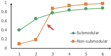
Despite evidence that many influence cascades display complex dynamics [Backstrom et al., 2006; Romero et al., 2011; Ugander et al., 2012], there are very limited studies on CCIM. Mainstream IM algorithms rely crucially on a property of simple contagions called submodularity, which intuitively reflects diminishing returns to the selection of additional seeds (the green curve in Figure 1). Under submodularity, a simple greedy algorithm is highly effective [Kempe et al., 2003]. However, the CC models' surge of cascade probability in adoption probability violates submodularity. This greatly complicates optimization by introducing complementarities: the marginal gain to selecting any single seed will often be small since its value is only revealed in combination with a specific set of other seeds. Formally, this means that CCIM is NP-hard to approximate even under simplified network models [Schoenebeck and Tao, 2019]. To our knowledge, the only practical algorithm for CCIM thus far is the Dynamic Programming for Influence Maximization (DPIM) approach of [Angell and Schoenebeck, 2017]. However, DPIM heavily relies on the assumption that the network has a hierarchical structure and its effectiveness may be limited when a good hierarchical decomposition cannot be found.
CCIM is essentially a stochastic combinatorial optimization problem (COP) with a non-submodular objective function. Inspired by recent works that use RL to address COPs [Bello et al., 2016; Khalil et al., 2017; Kool et al., 2018; Kwon et al., 2020], especially (submodular) influence maximization [Manchanda et al., 2020; Chen et al., 2021], we take a step further and ask the research question: Can we use RL to address complex contagion influence maximization?
The underlying idea of RL-based approaches to COPs is to decompose the original seed set selection into a sequence of seeds, and it does so greedily based on the marginal "score" of each node. The scores are estimated using deep function approximators. Despite the initial success of applying RL for IM, we found that directly applying these methods to the CCIM problems often yields suboptimal performance. A major challenge is that the reward signal in CCIM is much more sparse than simple contagion IM. We identify two distinct causes of reward sparseness. First, the effective solution space (i.e., solutions with non-negligible influence) is much smaller. This is because CC requires a harsher condition for influence to spread. Second, the marginal contribution of each node (action) in CCIM is more sparse than regular IM, because the reward becomes non-negligible only after multiple seeds are selected. This yields small or zero reward at the first few time steps even with the credit assignment mechanism used in previous works [Manchanda et al., 2020; Chen et al., 2021]. We refer to the two causes of reward sparseness as effective solution sparseness and credit sparseness.
To address the two issues, we propose a new RL-based solution approach called Reinforcement Learning for Influence Maximization with Complex Contagion (RL4CCIM), with several innovative components to existing approaches [Manchanda et al., 2020; Chen et al., 2021]. For effective solution sparseness, we design a solution filtering step that yields more effective policy exploration. We also use an adapted return-based prioritized experience replay (PER) [Schaul et al., 2016] component that increases the chances of sampling training transitions with higher rewards. For credit sparseness, we propose a new reward-shaping component which, at the end of each training episode, assigns an additional reward to nodes by looking at their marginal contribution w.r.t. the global action sequence.
Our main contributions are: 1) We propose the first learningbased approach to CCIM. Our work is also one of the first few that study CCIM and non-submodular IM. 2) We identify key challenges in applying existing RL approaches to the CCIM problem, and propose a novel RL algorithm to address them. 3) We conduct extensive empirical evaluations. Results on 9 realworld networks and various settings show that our approach achieves state-of-the-art performance. The effectiveness of our proposed components is shown via ablation study.
2 RelatedWork
Complex contagion influence maximization. [Domingos and Richardson, 2001] are the first to study the IM problem from an algorithmic perspective. [Kempe et al., 2003] formulate it as a discrete optimization problem on the networks, along with a greedy solution which has an approximation ratio of 1 - 1/e. The greedy algorithm is improved by various follow-up studies [Leskovec et al., 2007b; Borgs et al., 2014; Tang et al., 2015] which accelerate the algorithms with performance guarantees. These studies focus on cascade models such as IC and LT, which are essentially submodular. [Backstrom et al., 2006] show that influence diffusion models often appear to be "S-shaped" (see e.g. Figure 1), i.e., the probability of influence propagation has slow growth for small numbers of friends, rapid growth for a moderate numbers of friends, and a rapid flattening of the curve beyond a certain point. The phenomenon is further studied in the epical work [Centola and Macy, 2007] where the complex contagion model is introduced to model such collective social behavior, where the cascade probability is higher when multiple neighbors are activated. The model is validated by evidence from various succeeding studies [Leskovec et al., 2007a; Centola, 2010; Romero et al., 2011]. 1
Despite the broad existence of complex contagion, there have been extremely limited studies on the influence maximization problem from an algorithmic perspective. [Ghasemiesfeh et al., 2013; Gao et al., 2016] provide an analytical study of the complex contagion model given certain assumptions of the underlying network models. They do not consider the seed selection problem. [Schoenebeck and Tao, 2017; Schoenebeck and Tao, 2019] point out that the CCIM is nonsubmodular, and prove that it is NP-hard to approximate even under simplified network models. To our knowledge, [Angell and Schoenebeck, 2017] provide the only practical method that address the non-submodular IM problems via dynamic programming. However, their approach highly relies on the assumption that the networks are hierarchically structured, and therefore its performance heavily depends on the hierarchical decomposition component of the original network. A more recent study [Schoenebeck et al., 2020] prove theoretically the best seeding strategy on the stochastic hierarchical blockmodel, with other strong assumptions on the density of the network. Their seeding strategy has not been empirically evaluated. In contrast to the analytical approaches in existing works, we present the first learning based approach to CCIM.
RL for COPs. The key idea of RL based methods to COPs is to decompose the original combinatorial action into a sequence of individual actions, and then learn policies that greedily select nodes based on the "scores" estimated by deep function approximators [Bello et al., 2016; Graves et al., 2016]. Later approaches integrate RL with more sophisticated representation learning methods such as graph neural networks [Khalil et al., 2017], recurrent neural networks [Nazari et al., 2018], or attention mechanisms [Kool et al., 2018; Deudon et al., 2018] to better approximate the value/policy functions for COPs. The learning procedures are further augmented by additional beam search [Joshi et al., 2019], Monte Carlo tree search [Fu et al., 2021], dynamic programming [Kool et al., 2021], active search [Hottung et al., 2021], or multiple rollouts during inference [Kwon et al., 2020]. These techniques are then applied in various domains including scheduling in clusters [Mao et al., 2019], transportation [Qiu et al., 2019], job shop scheduling [Zhang et al., 2020], vehicle routing [Kool et al., 2021], network planning [Zhu et al., 2021] and epidemics control [Ou et al., 2021]. We refer to [Bengio et al., 2021; Mazyavkina et al., 2021] for a detailed survey.
1 The other variants of complex contagion [Ugander et al., 2012; Banerjee et al., 2013] are out of scope of this paper.
RL for IM. Early attempts of RL for IM problems [Lin et al., 2015; Ali et al., 2018] focus on learning which high-level greedy algorithm to use, instead of the specific seeding strategy. [Kamarthi et al., 2020] apply RL to explore the structure of an unknown network in influence maximization, instead of the seeding strategy. [Li et al., 2019; Tian et al., 2020; Manchanda et al., 2020; Chen et al., 2021] extend the method in [Khalil et al., 2017] to address the IM problem, where to address the credit assignment problem, the reward of a new node is defined as its marginal contribution. [Manchanda et al., 2020] focus on solving IM problem instances with very large networks. [Chen et al., 2021] use RL to address IM problem where the willingness of a node to be a seed is uncertain. To the best of our knowledge, none of them consider CCIM, which is much more challenging compared to classic IM because of non-submodularity and the resulting reward sparseness issues.
3 Complex Contagion Influence Maximization
We consider a social network as a graph G = (V, E), where V and E are the nodes and edges, respectively. Each node is either activated or inactivated, which means the node is influenced or not. We assume all nodes are initially inactivated unless chosen as the seed node. Nodes which are linked by edges have a probability p of influencing each other. For each node v, its neighbors are represented as N(v). In simple contagions such as the Independent Cascade (IC) model [Goldenberg et al., 2001] and the Linear Threshold (LT) model [Granovetter, 1978], the probability p is assumed to be a constant that is independent of the number of its neighbors 2 . In complex contagion, the assumption is relaxed, and p is represented as a dependent variable of the number of activated neighbors k. Without loss of generality, we consider the most classical K-complex contagion model [Centola and Macy, 2007; Centola, 2010; Ghasemiesfeh et al., 2013], where
where 0 ≤ p1 ≪ p0 ≤ 1. p1 (p0) can be interpreted as a very small (large) influence probability when there is a small (large) number of activated neighbors. K ≥ 1 is an integer threshold value. K is interpreted as the threshold to make a qualitative change to p(k). Given a set S ⊆ V of seed nodes, the influence of the complex contagion is represented as σ(G, S). The complex contagion influence maximization problem is to select the optimal set of seeds S∗ such that the influence is maximized:
2 By LT, we refer to the canonical version where the activation threshold is uniformly distributed in [0,1], which is submodular. In LT models, p can be seen as the weight that an activated neighbor adds to the target node.
given |S| = T, i.e., the number of seeds is equal to budget T. Definition 1. A set function f : 2V →R is submodular if for any S ⊂ S′ ⊂ V and any v ∈ V \ S′ , it holds that
Theorem 1. The influence function σ(G, S) defined based on the cascade probability function in Equation.(1) is nonsubmodular.
See proof in Appendix A. Because Independent Cascade (IC) IM is NP-hard [Kempe et al., 2003], we have
Theorem 2. The K-complex contagion influence maximization problem is NP-hard.
The proof can be done by showing that a special instance of K-complex contagion is an arbitrary instance of the IC model. Consider a special instance of K-complex contagion when K = 1. In this instance, the cascade probability p(k) in Eq.(1) becomes a constant value that does not depend on k: p(k) = p0. In other words, it is equivalent to an arbitrary instance of the IC model.
Non-submodular models are fundamentally harder than submodular ones because the algorithm needs to take exactly the right combination of nodes before receiving any reward; the individual actions may fail to generate any influence on their own. For submodular models, there are no such "complementarities" between nodes and so greedy strategies are provably optimal. An advantage of RL over other heuristics is that during training it looks ahead multiple steps (guided by the exploration policies, the n-step return, and the intermediate rewards we propose) instead of being trapped in a bad local optimum like greedy methods. Another strength of RL is that it can learn policies to any given network structure without redesigning the solution architecture.
Therefore, inspired by recent works that combine RL and graph representation techniques to address COPs on graphs [Khalil et al., 2017; Deudon et al., 2018; Bengio et al., 2021] and influence maximization in particular [Manchanda et al., 2020; Chen et al., 2021], we design a new RL algorithm to address the CCIM problem, called Reinforcement Learning for Complex Contagion Influence Maximization (RL4CCIM).
4 MDP Formulation &RL Preliminary
4.1 MDP Formulation of CCIM
In order to fit the complex contagion influence maximization problem into the RL framework, we first formulate this problem as a discrete time MDP. In this MDP, the time steps t = 1 . . . T correspond to the sequence of seed node selections. That is, each time step t means selecting one seed node, and the time horizon of the MDP is the total budget T .
The state captures the current status of a node selection time step t, i.e., which nodes have already been selected before t. We use a binary indicator vector Xt ∈ {0, 1}|V | to represent the state, where an element Xt,v = 1 means the node v is selected (activated), and 0 otherwise. It is easy to see that ∑|V | v=1 Xt,v = t-1, i.e., the total number of selected nodes at time t is equal to t-1. Here Xt can be seen as the vector-form equivalence of the set-form notation St (i.e., the set of nodes selected as seeds at time t).
Given state Xt at time t, the action at is to select the next node. We use a one-hot vector at ∈ {0, 1}|V | to represent the action, where the non-zero element at,v = 1 means node v is the selected node at the current time step. The transition function is represented as
It is worth noting that the transition function in this setting is deterministic. The terminal state XT is the state at the final time step T , and it suffices that ∑|V | v=1 XT,v = T . Following the ideas in [Manchanda et al., 2020; Chen et al., 2021], the one-step reward is defined as the marginal contribution of a new seed node selected at time t, i.e.,
where σ(G,Xt) is equivalent to the set-form notation σ(G, St), with St being the set of seeds selected at t.
4.2 RL Preliminaries
RL is a learning paradigm where agents learn to take actions in an environment to achieve a certain goal. In this paper, the environment is the MDP that we formulated previously. At each time step t of the MDP, the agent takes an action based on its policy π(at|Xt), where Xt and at are respectively the state and action of the MDP. The selected action then interacts with the environment and the environment returns a reward signal rt(Xt, at) which reflects how good the action/policy is, as well as the next state Xt+1. Q-learning [Watkins and Dayan, 1992] is a value-based RL variant that represents the value of a state action pair (Xt, at) with the Q-function Q(Xt, at). The Q-function is usually updated using the Bellman equation: Q(Xt, at) = rt(Xt, at) + γ maxat+1 Q(Xt+1, at+1), where γ is the discount factor. During training, actions are usually taken by balancing the exploitation which takes the action with the highest Q-value, and exploration which takes a random action (usually with a decaying probability ε). DQN [Mnih et al., 2013] improves Q-learning's function approximator with parameterized deep neural networks Qθ(Xt, at), together with adoption of other techniques including the ideas of experience replay [Lin, 1992], which stores the training trajectories in a replay buffer and then updates the neural networks parameters θ using mini-batches of data. In this paper, we use the doubleDQN framework [Van Hasselt et al., 2016] as our base RL method which trains an additional target network to mitigate the overestimation issue in vanilla DQN.
5 RL4CCIM
We first use a motivating example that illustrates the reward sparseness issues. We then introduce the key methodology.
5.1 AMotivating Example
Recent studies [Khalil et al., 2017; Kwon et al., 2020] integrate RL with deep function approximators to address combinatorial optimization over graphs, including influence maximization [Manchanda et al., 2020; Chen et al., 2021]. We build RL4CCIM on this line of works. Despite the initial success of these methods in generic COPs and IM problems, we found that the non-submodularity of the CC models and the resulting reward sparseness creates a major hurdle that prevents us from directly applying these existing methods.
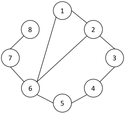
More specifically, the reward sparseness arises from two causes: the effective solution sparseness and credit sparseness. To take a closer look at the two issues, we refer to the example network in Figure 2 with a standalone illustration. Set p0 = 1, p1 = 0, K = 3 in Eq.(1), and the budget as T = 4. There are in total C 4 8 = 70 feasible solutions. (i) Effective solution sparseness. For simple contagion (i.e., K = 1) where p(k) = p0 = 1, because it is a fully connected network, any solution is an effective solution. Whereas for the complex contagion (K = 3), only nodes 2 and 6 have at least 3 neighbors, and therefore can be activated when there are enough activated neighbors. Many solutions (e.g., {5, 6, 7, 8} or {1, 2, 3, 4}) are ineffective which cannot activate any other node. Using exhaustive search, we can get that there are 17 out of C 4 8 = 70 combinations of 4 seeds that are effective solutions, taking up only 24.3%. (ii) Credit sparseness. We consider a sequence of seed nodes: {1, 2, 3, 5}. It is an effective solution which can activate node 6. However, because of the way the reward is defined (see Eq.(4)), the reward of the first three steps are all 1's (i.e., only the seed node itself is activated), and only the last time step has a reward of 2. This leads to very slow training since the first time steps yield the same reward of 1.
5.2 RL4CCIMArchitecture
The above two issues motivate the design of RL4CCIM. Figure 3 shows the overall architecture of RL4CCIM, where the key novelties are i) a solution filtering mechanism that provides a warm-start of the learning procedure, ii) a customized prioritized experience replay component that encourages training transitions with higher rewards, and iii) a reward shaping component which mitigates the assignment sparseness issue. Algorithm 1 presents the training algorithm of RL4CCIM, which follows the flow of DQN, with the 3 new elements being described in: Lines 3-5 and 9 for solution filtering, Line 11 for PER, and Lines 13-16 for reward shaping.
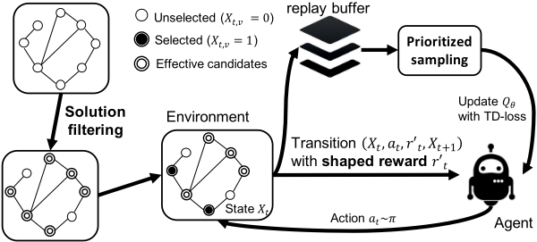
As a fourth improvement, instead of using S2V [Dai et al., 2016] as the function approximator that works as the graph representation learning unit in [Khalil et al., 2017] and RL4IM [Chen et al., 2021], we use a more advanced graph representation learning technique called graph attention networks (GAT) [Veliˇckovi´c et al., 2018]. GAT is a neural network architecture that operates on graph-structured data, leveraging masked self-attentional layers [Vaswani et al., 2017] to address the shortcomings of prior methods based on graph convolutions or their approximations. We focus on the elaboration of the first three improvements and refer to the original paper [Veliˇckovi´c et al., 2018] for a detailed description of GAT.
Algorithm 1: RL4CCIM training
1 Input: network G = (V,E), seed budget T, complex contation paramters p0, p1, K 2 Initialize Qθ(·) and replay bufferM← ∅ 3 Initialize A← ∅ 4 for v ∈ V do 5 if |N(v)| ≥K then A←A∪N(v); 6 for episode = 1 . . . E do 7 Reset environment, initialize state X1 ← 0 8 for t = 1 . . . T do 9 With probability 1 - ε take action at ← arg maxat∈ Qθ(Xt, at); with probability ε ∗ ε′ take a random action at ∈ {0, 1}|A| ; with probability ε(1 - ε′ ) take a random action at ∈ {0, 1}|V | 10 Get new transition m ← (Xt, at, rt, Xt+1), where rt is calculated with Eq.(4). 11 Sample mini-batch data M ⊂ M with Eq.(5) 12 Update Qθ with M using gradient descent 13 for t = 1 . . . T do 14 Calculate r′ (Xt, at) with Eq.(7) 15 Get shaped transition m′ ← (Xt, at, r′t, Xt+1) 16 Update replay buffer M ← M ∪ m′ 17 return Qθ(·)5.3 Solution Filtering
As introduced previously, a main challenge in applying existing RL for IMmethods is the effective solution sparseness.
Definition 2 (Effective solution). Given G and σ(G, S), an effective solution is a solution S where σ(G, S) > |S|.
For a network G = (V,E) and a budget of T, the size of the feasible solution space is then C T |V | , the complexity of which is O( min(|V |T , |V ||V |-T )). While the sequence decomposition avoids enumerating the combinatorial action space, the effective solutions are in fact very sparse in the CCIM problem. This makes initial learning very slow as most episodes have close to 0 rewards. For instance, only 24.2% of nodes in the toy example in Figure 2 have non-zero rewards. The percentage of effective solutions gets even lower when the network sizes and the threshold K are larger.
To that end, our key observation is that certain nodes are never part of an effective solution. For example, nodes 4 and 8 are never able to activate any other nodes. Thus, we may remove them from the feasible solution space to increase the chances that effective solutions are selected. In doing so, the number of feasible solutions becomes C 4 6 = 15, which is 15/70 = 21.4% of the original feasible solution space.
Inspired by this, we design a solution filtering mechanism, as described in Lines 3-5 of Algorithm 1. We initialize an empty node set A = ∅ which stores the set of filtered nodes that could potentially be selected as seed nodes. We enumerate through each node v ∈ V of a network, and check if the number of its neighbors is no smaller than the threshold K. If it is, then we update A as the union of A and all the neighbors of v. In this case, if a node is not in any neighborhood which can potentially activate another node, that node will not be contained in the effective candidate set A. Because of this, it is guaranteed that
Theorem 3. The effective candidate set A contains any effective solution S where σ(G, S) > |S|.
This means that the solution filtering step does not exclude any potentially optimal solution. When exploring new actions, instead of taking a random action from the entire action space
{0, 1}|V | , the action exploration in RL4CCIM is initially restricted on {0, 1}|A| (Line 9). To ensure that the solution space is sufficiently explored and un-biased in the final stage, we use an annealing factor (similar to the original exploration probability ε) ε′ that gradually deceases from a large value (e.g., 0.99) to a small value (e.g., 0). The probability of selecting from the effective candidate set A is then ε ∗ ε′ .
5.4 Reward-based Prioritized Experience Replay
The solution filtering mechanism does not guarantee that any combination of solution in A is effective. E.g., in Figure 2, if there is a node 9 which is only linked to node 3, then A = {1, 2, 3, 4, 5, 6, 7, 9}. However, solution {1, 2, 6, 9} does not activate any other node and thus is not an effective solution.
The solution filtering mechanism works at the generation time of training trajectories. All the transitions generated will be stored into the replay buffer and later used to sample batches of training data. To further encourage sampling effective solutions, or more specifically, solutions with higher rewards, we adopt the idea of Priotized Experience Replay (PER) [Schaul et al., 2016]. Opposed to sampling transition data uniformly in classical experience replay [Lin, 1992], PER samples transition data with different priorities defined based on a certain metric.
In [Schaul et al., 2016], the selection metric is defined as the temporal difference (TD) error δ = rt(Xt, at) + γ maxat+1 Q(Xt+1, at+1) - Qθ(Xt, at). Let qi = |δi| + ϵ, where ϵ > 0 is a very small value to prevent 0 in the denominator, the probability of sampling a trajectory i with TD error δi is then Pi = qα i ∑k qα k , where α is a temperature parameter.
In RL4CCIM, because we aim to increase the chances of sampling transitions with higher rewards, we propose two other versions of priority values. One version is to directly use reward 3 ri(X, a) as the priority value: pi = ri(X, a) + ϵ. Though this encourages transitions with higher rewards, it has the risk of causing overestimation, where the biases of rewards are exaggerated by the Bellman target [Van Hasselt et al., 2016]. Indeed, we found that in practice, this version is sometimes not stable. We therefore introduce a third variant which takes the (weighted) sum of them qi = |δ|+βri(X, a)+ ϵ. The sampling probability is then:
This form of priority balances the benefit of training with high reward transitions and the risk of overestimating Q values.
5.5 Reward Shaping
As shown in Eq. (4), existing RL for IMmethods define the reward of a new seed node at as the marginal contribution of that node w.r.t. its "preceding" seeds Xt = ∑t-1 τ=1 aτ . This is reasonable when the influence function is submodular - because the following nodes will make smaller marginal contributions. This becomes insufficient when it comes to complex contagion, where the influence function is no-longer submodular. As illustrated in Section 5.1, this incurs the credit sparseness issue.
3 In practice, we use the "n-step" return [Watkins, 1989] instead because it can look at more steps of reward in the future, but omit the discussions here for ease of reading.
To mitigate this issue, our idea is to add a regularization term to the reward, which accounts for its marginal contribution (which is much more likely to be non-zero) from a "global" perspective. At first thought, the most desirable regularization is the Shapley value [Shapley, 2016]. This, however, introduces exponentially large number of calculations of marginal contributions, which is computationally infeasible. As a simplified alternative, we use the marginal contribution of action at w.r.t. the sequence of nodes selected in the same episode:
where a1:t := ∑tτ=1 aτ . a1:t-1 and at+1:T respectively represent preceding and proceeding seed nodes of at. The shaped reward is then represented as:
where ω is the weight. Note that this requires running an entire simulation before assigning the immediate reward of each action/seed (see Lines 13-16 of Algorithm 1).
6 Experiments
We first present evaluations of the performances of RL4CCIM and baselines on various real-world networks and problem settings. We then do an ablation study to evaluate the effectiveness of the components that we introduce in Section 5. All experiments are run on a Dell DSS 8440 Cauldron node, with a virtual environment, 2 Intel Xeon Gold 6148 2.4G CPU cores, 5G RAM, 1 NVIDIA Tesla V100 32G GPU, EDR Infiniband.
We consider the following baselines: (i) Random+, which selects seeds randomly from the effective candidate set A, (ii) Greedy [Kempe et al., 2003], which is the prominent approach for submodular IM, (iii) DPIM [Angell and Schoenebeck, 2017], which is a dynamic programming based method designed for non-submodular IM including CCIM. To the best of our knowledge, this method is the only published method for non-submodular IM. Note that the code of DPIM is not publicly available. Therefore we implemented our own version of DPIM, where to build a hierarchical decomposition tree of the original network, we use the Jaccard Similarity variant (see Section 4.1.3 of [Angell and Schoenebeck, 2017]). Our implementation of DPIM is in the supplementary material, and we plan to open-source it at the time of publication. (iv) RL4IM [Chen et al., 2021], which is the most recent work that uses RL for submodular IM.The hyper-parameter values selected and ranges that are searched within for different methods are described in Appendix B.
To have a sense of the optimality gap of the different methods (on small networks), we also implemented a Mixed Integer Programming (MIP) based optimization approach (shown as the last row "OPT" of Table 1) using the Gurobi solver. The detailed description of the formulation is in Appendix D. While MIP finds the exact optimum, its runtime increases rapidly with the network size. We set a 12 hour time limit, which was exceeded starting at Network SPY (67 nodes). We also found that in stochastic settings MIP was too expensive to solve even for small networks. This shows that CCIM is too difficult for existing generic optimization approaches.
| Method \ Network | CHANGE | DC | DOSIM | MFP | SPY | Football | Polbooks | India | Exhibition |
|---|---|---|---|---|---|---|---|---|---|
| Greedy | 0.1509 | 0.3902 | 0.225 | 0.3194 | 0.4925 | 0.3217 | 0.4571 | 0.0396 | 0.0293 |
| DPIM | 0.283 | 0.4146 | 0.35 | 0.2917 | 0.477 | 0.3913 | 0.6762 | 0.3911 | 0.5537 |
| Random+ | 0.1632 | 0.3049 | 0.2175 | 0.1313 | 0.2955 | 0.0926 | 0.1486 | 0.0498 | 0.0293 |
| RL4IM | 0.283 | 0.4146 | 0.325 | 0.3194 | 0.4925 | 0.513 | 0.7429 | 0.3465 | 0.5439 |
| RL4CCIM | 0.283 | 0.4634 | 0.375 | 0.3472 | 0.5075 | 1.0 | 0.819 | 0.5347 | 0.5585 |
| OPT | 0.3019 | 0.4634 | 0.375 | 0.375 | 0.5522 | N/A | N/A | N/A | N/A |
We evaluate different methods on a set of 9 real-world networks. These include 5 small social-networks that are collected from homeless youth shelters in the city of Los Angeles. They are denoted as CHANGE, DC, DOSIM, MFP, SPY. We also evaluate on 4 publicly available and larger sized real-world networks, including Football [Girvan and Newman, 2002], Polbooks [Rossi and Ahmed, 2015], India [Banerjee et al., 2013], and Exhibition [Isella et al., 2011]. The detailed description of the networks is presented in Appendix C. Note that training time and scalability are not the focus of our work, so all experiments are run on small-sized networks. Training of all RL-based methods finishes within 2 hours.
6.1 Comparing with Baselines
In the basic problem setting, we set propagation probabilities p1 = 0, p0 = 1, so that the propagation is deterministic. This setting is convenient for comparison as it rules out the factor that arises from stochasticity of different runs. We will show results later in a setting with stochastic propagation. The threshold K values are set to 3 for small networks CHANGESPY, 4 for medium networks (Football, Polbooks and India), and 6 for the largest network Exhibition. The values are set as such so that the influence spread is neither too sparse (very few nodes are influenced) nor too dense (most nodes are influenced) where comparisons become trivial. In this set of experiments, we set the seed budget T = 8 for all the networks except for the largest network Exhibition which is T = 12. In deterministic settings, there is no randomness for Greedy and DPIM. Randomness of Random+ and RL methods arises from different running seeds. For Random+, we run 50 times each and take the average. For RL methods, we run 15 times and find the best model via a separate validation process (performs every 20 training time steps), and report its performance.
We have these observations in Table 1. (i) RL4CCIM consistently obtains the best results among all the methods across all the 9 networks. It obtains the optimal or closeto-optimal solutions on small networks. (ii) The Random+ method, though being far from optimal, seems to be sufficient to serve as a warm-start for RL4CCIM. (iii) Surprisingly, Greedy can be arbitrarily bad. For example, Greedy obtains only an influence value of 0.0396 on the India network. Considering that there are 202 nodes in this network, this means that Greedy does not find any effective solution. To better understand this, we compare the seeds selected by Greedy and RL4CCIM on the India network in Figure 6 of Appendix E. (iv) RL4IM and DPIM are unstable. RL4IM achieves influence values close to RL4CCIM on some networks (e.g., CHANGE, SPY, and Exibition). However, on some other networks, especially relatively large networks (Football, Polbooks, and India), it is significantly beaten by RL4CCIM. Our hypothesis is that the effective solution sparseness becomes more severe when the entire solution space grows larger. The same holds for DPIM, where it works well on networks such as CHANGE and Exhibition, but is much worse than RL4CCIM on some other networks (e.g., Football and India). A main reason, in our understanding, is that DPIM highly relies on the assumption that networks are hierarchically structured, and therefore the performance of it highly depends on how the network's structure is aligned with the assumption. Unfortunately in practice, it is hard to measure the hierarchy of networks.
6.2 Evaluation on Various Other Problem Settings
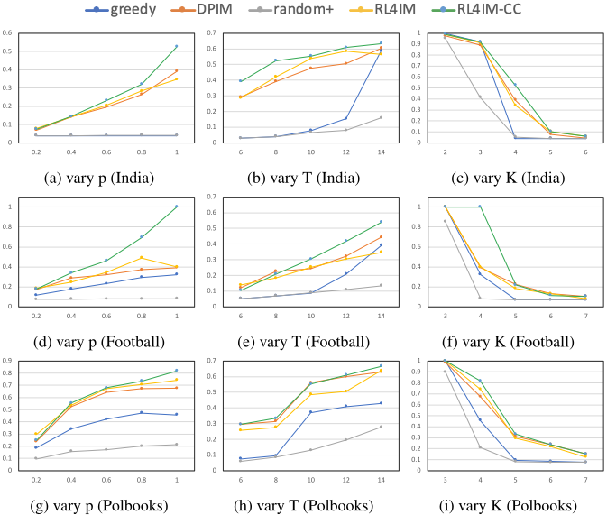
We are also interested to see how different methods work under a variety of other problem settings, including: (a) Stochastic propagation. We set the range of p1 as [0.2, 0.4, 0.6, 0.8, 1]. In the stochastic setting, we also run Greedy and DPIM for 20 times and report the average. (b) Seed budget T. We set the range of T as [6, 8, 10, 12, 14]. (c) Activation threshold K. We set its range as [2, 3, 4, 5, 6]. When evaluating changing T in Football, we set K = 5 instead of 4 as k = 4 immediately yields influence value of 1 for RL4CCIM (see for example Figure 4f) and thus the comparison becomes trivial.
We evaluate the different settings on three networks, including India, Football, and Polbooks. The results are shown in Figure 4. We can notice that the trends on different networks are consistent. For example, Figures 4(a)-(c) show the results on the India network. We can see that: (i) In all of the settings, RL4CCIM still consistently outperforms all the baselines. This shows the robustness of RL4CCIM. (ii) It follows the intuition that the influence value is higher when there is a higher propagation probability p, a larger number of seeding budget T, and a smaller threshold K. (iii) Interestingly, there is a surge of influence value for Greedy when the seed budget T increases from 12 to 14, and when the threshold K decreases from 4 to 3. Our hypothesis is that when T becomes larger (or K becomes smaller), the ratio of effective solutions becomes much larger, and therefore the estimation of marginal influence w.r.t. a set of nodes for Greedy becomes much more accurate. However, both of the situations essentially come at the cost of a large seed budget.
6.3 Ablation Study
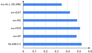
To evaluate the effectiveness of the different customized components, we also conduct an ablation study on the India network, using the basic problem setting. In each comparison, we remove one of the 4 components, and get 4 versions of RL4IMC-CC, namely 1) wo-SF (without solution filtering), 2) wo-PER (without prioritized experience replay), 3) wo-RS (without reward shaping), 4) wo-GAT ((without GAT, using S2V instead). Finally, we also show the version without any of these components (wo-ALL), which reduces to RL4IM. The comparison is shown in Figure 5. We can see that by removing each of the components, there is a substantial decrease in the normalized influence value, respectively 10.2% (wo-SF), 4.6% (wo-PER), 9.3% (wo-RS), and 21.3% (wo-GAT). When removing the 3 components altogether, there is a largest decrease of 35.2%. These results demonstrate the importance of all the four additional components.
Limitation Though our method works well on the smaller networks, scalability is a major limitation of the current version. The main bottlenecks of scaling up are (roughly) twofold: (1) Simulation time of complex contagion. Simulation time is the top bottleneck as RL needs sufficient training episodes. For simple contagion models which are much better studied, there have been efficient methods that can accelerate the simulation (e.g., [Wang et al., 2012]). Complex contagion on the contrary, has been less studied. Hence less effort has been put on improving the simulation efficiency of complex contagion, partly also due to the fact that complex contagion is more challenging to simulate. (2) RL training. On the other hand, gradient updates in Q-networks take more time and memory as it requires larger scale matrix computation. To overcome this issue, a solution is to do pre-processing of the large networks. For example, we may scale them down by pruning less important/informative nodes from the original networks (e.g., the idea from [Manchanda et al., 2020]).
7 Conclusion
We propose the first learning-based approach to CCIM, with multiple innovative components that exploit the structure of the CCIM problem. Empirical results show that our approach achieves new state-of-the-art performance in CCIM. Our work opens up many potential future directions for learning-based approach to CCIM. For example, it is interesting to explore: (i) Can we design more efficient RL algorithms for larger networks? (ii) Can the learned RL policies generalize to new networks? (iii) What if the network structures or the complex contagion model parameters are uncertain?
Acknowledgments
This work was supported by the Army Research Office (MURI W911NF1810208). Bo An is supported by the National Research Foundation, Singapore under its Industry Alignment Fund - Pre-positioning (IAF-PP) Funding Initiative. Any opinions, findings and conclusions or recommendations expressed in this material are those of the author(s) and do not reflect the views of National Research Foundation, Singapore.
@inproceedings{ijcai2023p614,
  title     = {Complex Contagion Influence Maximization: A Reinforcement Learning Approach},
  author    = {Chen, Haipeng and Wilder, Bryan and Qiu, Wei and An, Bo and Rice, Eric and Tambe, Milind},
  booktitle = {Proceedings of the Thirty-Second International Joint Conference on
               Artificial Intelligence, {IJCAI-23}},
  publisher = {International Joint Conferences on Artificial Intelligence Organization},
  editor    = {Edith Elkind},
  pages     = {5531--5540},
  year      = {2023},
  month     = {8},
  note      = {Main Track},
  doi       = {10.24963/ijcai.2023/614},
  url       = {https://doi.org/10.24963/ijcai.2023/614},
}
TY - CPAPER TI - Complex Contagion Influence Maximization: A Reinforcement Learning Approach AU - Chen, Haipeng AU - Wilder, Bryan AU - Qiu, Wei AU - An, Bo AU - Rice, Eric AU - Tambe, Milind T2 - Proceedings of the Thirty-Second International Joint Conference on Artificial Intelligence, IJCAI-23 PB - International Joint Conferences on Artificial Intelligence Organization PY - 2023 SP - 5531 EP - 5540 DO - 10.24963/ijcai.2023/614 UR - https://doi.org/10.24963/ijcai.2023/614 ER -Copied
Machine-readable versions of this paper, for tools and AI agents:





