
On Tackling Explanation Redundancy in Decision Trees (Extended Abstract)
Proceedings of the Thirty-Second International Joint Conference on Artificial Intelligence. Journal Track. Pages 6900-6904.
https://doi.org/10.24963/ijcai.2023/779
Keywords
- Machine Learning: ML: Symbolic methods
- Knowledge Representation and Reasoning: KRR: Diagnosis and abductive reasoning
- AI Ethics, Trust, Fairness: ETF: Trustworthy AI
- Machine Learning: ML: Explainable/Interpretable machine learning
- Constraint Satisfaction and Optimization: CSO: Constraint satisfaction
- Knowledge Representation and Reasoning: KRR: Automated reasoning and theorem proving
- Constraint Satisfaction and Optimization: CSO: Satisfiabilty
Abstract
Claims about the interpretability of decision trees can be traced back to the origins of machine learning (ML). Indeed, given some input consistent with a decision tree's path, the explanation for the resulting prediction consists of the features in that path. Moreover, a growing number of works propose the use of decision trees, and of other so-called interpretable models, as a possible solution for deploying ML models in high-risk applications. This paper overviews recent theoretical and practical results which demonstrate that for most decision trees, tree paths exhibit so-called explanation redundancy, in that logically sound explanations can often be significantly more succinct than what the features in the path dictates. More importantly, such decision tree explanations can be computed in polynomial-time, and so can be produced with essentially no effort other than traversing the decision tree. The experimental results, obtained on a large range of publicly available decision trees, support the paper's claims.
- [Amgoud, 2021] Leila Amgoud. Non-monotonic explana- tion functions. In ECSQARU, pages 19-31, 2021.
- [Arenas et al., 2022] Marcelo Arenas, Pablo Barceló, Miguel Romero, and Bernardo Subercaseaux. On com- puting probabilistic explanations for decision trees. In NeurIPS, 2022.
- [Audemard et al., 2020] Gilles Audemard, Frédéric Koriche, and Pierre Marquis. On tractable XAI queries based on compiled representations. In KR, pages 838-849, 2020.
- [Audemard et al., 2021] Gilles Audemard, Steve Bellart, Louenas Bounia, Frédéric Koriche, Jean-Marie Lagniez, and Pierre Marquis. On the computational intelligibility of boolean classifiers. In KR, pages 74-86, 2021.
- [Barceló et al., 2020] Pablo Barceló, Mikaël Monet, Jorge Pérez, and Bernardo Subercaseaux. Model interpretability through the lens of computational complexity. In NeurIPS, 2020.
- [Bertsimas and Dunn, 2017] Dimitris Bertsimas and Jack Dunn. Optimal classification trees. Mach. Learn., 106(7):1039-1082, 2017.
- [Breiman et al., 1984] Leo Breiman, J. H. Friedman, R. A. Olshen, and C. J. Stone. Classification and Regression Trees. Wadsworth, 1984.
- [Breiman, 2001] Leo Breiman. Statistical modeling: The two cultures. Statistical science, 16(3):199-231, 2001.
- [Darwiche and Hirth, 2020] Adnan Darwiche and Auguste Hirth. On the reasons behind decisions. In ECAI, pages 712-720, 2020.
- [Ghiasi et al., 2020] Mohammad M. Ghiasi, Sohrab Zende- hboudi, and Ali Asghar Mohsenipour. Decision tree-based diagnosis of coronary artery disease: CART model. Com- put. Methods Programs Biomed., 192:105400, 2020.
- [Gorji and Rubin, 2022] Niku Gorji and Sasha Rubin. Suf- ficient reasons for classifier decisions in the presence of domain constraints. In AAAI, February 2022.
- [Hu et al., 2019] Xiyang Hu, Cynthia Rudin, and Margo I. Seltzer. Optimal sparse decision trees. In NeurIPS, pages 7265-7273, 2019.
- [Huang et al., 2021] Xuanxiang Huang, Yacine Izza, Alexey Ignatiev, and Joao Marques-Silva. On efficiently explain- ing graph-based classifiers. In KR, pages 356-367, 2021.
- [Huang et al., 2022] Xuanxiang Huang, Yacine Izza, Alexey Ignatiev, Martin C. Cooper, Nicholas Asher, and Joao Marques-Silva. Tractable explanations for d-DNNF clas- sifiers. In AAAI, February 2022.
- [Ignatiev and Marques-Silva, 2021] Alexey Ignatiev and Joao Marques-Silva. SAT-based rigorous explanations for decision lists. In SAT, pages 251-269, 2021.
- [Ignatiev et al., 2019] Alexey Ignatiev, Nina Narodytska, and Joao Marques-Silva. Abduction-based explanations for machine learning models. In AAAI, pages 1511-1519, 2019.
- [Ignatiev et al., 2020] Alexey Ignatiev, Nina Narodytska, Nicholas Asher, and Joao Marques-Silva. From con- trastive to abductive explanations and back again. In AIxIA, pages 335-355, 2020.
- [Ignatiev et al., 2022] Alexey Ignatiev, Yacine Izza, Peter Stuckey, and Joao Marques-Silva. Using MaxSAT for ef- ficient explanations of tree ensembles. In AAAI, February 2022.
- [Izza and Marques-Silva, 2021] Yacine Izza and Joao Marques-Silva. On explaining random forests with SAT. In IJCAI, pages 2584-2591, 2021. IJCAI
- [Izza et al., 2020] Yacine Izza, Alexey Ignatiev, and Joao Marques-Silva. On explaining decision trees. CoRR, abs/2010.11034, 2020.
- [Izza et al., 2022] Yacine Izza, Alexey Ignatiev, and Joao Marques-Silva. On tackling explanation redundancy in de- cision trees. J. Artif. Intell. Res., 75:261-321, 2022.
- [Lelis et al., 2020] Viviane Maria Lelis, Eduardo Guzmán, and María-Victoria Belmonte. Non-invasive meningitis diagnosis using decision trees. IEEE Access, 8:18394- 18407, 2020.
- [Lin et al., 2020] Jimmy Lin, Chudi Zhong, Diane Hu, Cyn- thia Rudin, and Margo I. Seltzer. Generalized and scalable optimal sparse decision trees. In ICML, pages 6150-6160, 2020.
- [Liu and Lorini, 2021] Xinghan Liu and Emiliano Lorini. A logic for binary classifiers and their explanation. In CLAR, 2021.
- [Marques-Silva and Ignatiev, 2022] Joao Marques-Silva and Alexey Ignatiev. Delivering trustworthy AI through formal XAI. In AAAI, 2022.
- [Marques-Silva, 2022] Joao Marques-Silva. Logic-based ex- plainability in machine learning. CoRR, abs/2211.00541, 2022.
- [Molnar, 2020] Christoph Molnar. Interpretable Machine Learning. Leanpub, 2020. http://tiny.cc/6c76tz. Link
- [Quinlan, 1986] J. Ross Quinlan. Induction of decision trees. Mach. Learn., 1(1):81-106, 1986.
- [Rudin, 2019] Cynthia Rudin. Stop explaining black box machine learning models for high stakes decisions and use interpretable models instead. Nature Machine Intelligence, 1(5):206-215, 2019.
- [Shih et al., 2018] Andy Shih, Arthur Choi, and Adnan Dar- wiche. A symbolic approach to explaining bayesian net- work classifiers. In IJCAI, pages 5103-5111, 2018. IJCAI
- [Utgoff et al., 1997] Paul E. Utgoff, Neil C. Berkman, and Jeffery A. Clouse. Decision tree induction based on effi- cient tree restructuring. Mach. Learn., 29(1):5-44, 1997.
- [Verwer and Zhang, 2019] Sicco Verwer and Yingqian Zhang. Learning optimal classification trees using a binary linear program formulation. In AAAI, pages 1625-1632, 2019.
References were extracted automatically from the PDF and may contain errors.
Full text extracted automatically from the PDF; figures, tables and equations may differ. The PDF is the version of record.
1 Introduction
Since the inception of the first decision tree (DT) construction algorithms [Breiman et al., 1984; Quinlan, 1986], interpretability of DTs has been taken for granted. For example, a well-known researcher in ML, L. Breiman, once remarked that: "On interpretability, trees rate an A+" [Breiman, 2001] (page 206). More importantly, a number of recent works propose the use of interpretable models as an alternative to blackbox inscrutable ML models [Rudin, 2019; Molnar, 2020]. In addition, the small size/depth of DTs is often one of the main arguments supporting the learning of optimal decision trees [Bertsimas and Dunn, 2017; Hu et al., 2019; Verwer and Zhang, 2019; Lin et al., 2020]. It is usually implicit that the explanation in the case of a decision tree is the path consistent with the target instance.
However, the belief about the interpretability of decision trees is in fact a misconception. First, there are many examples of deployed decision trees that are both large and deep (e.g. [Ghiasi et al., 2020]). Second, and far more important, paths in decision trees can include nodes (and therefore literals) that are irrelevant for the prediction [Izza et al., 2022; Huang et al., 2021; Izza et al., 2020]. This last result was complemented by a number of additional theoretical and practical results. First, we proved that the number of redundant features can grow with the number of features, and that this is true even for size-optimal DTs. Second, we proved that DTs that do not have paths with explanation-redundant literals represent a very restricted class of DTs. Third, we showed experimentally that a large number of example DTs, used in publications since the inception of DT learning algorithms, exhibit explanation redundancy. Such publications include seminal papers on the induction of DTs, but also some of the best-known textbooks in AI/ML. Fourth, and finally, we showed experimentally that, without exception, DTs learned by well-known tree-learning tools will exhibit explanation redundancy, and that such explanation redundancy can be nonnegligible.
∗The full version is published in J. Artif. Intell. Res., 75:261-321, 2022.
This paper offers a brief overview of the results in [Izza et al., 2022]. Section 2 introduces the definitions and notation used throughout the paper. Section 3 summarizes the main contributions in [Izza et al., 2022]. Section 4 offers a brief perspective on the experimental results in [Izza et al., 2022]. Finally, Section 5 concludes the paper.
2 Preliminaries
Classification in ML. Classification problems are defined on a set of features F = {1, . . . ,m} and a set of classes K = {c1, . . . , cK}. Each feature i ∈ F takes values from a domain Di, where domains can be categorical or ordinal. Feature space is the cartesian product of the domains of the features, F = D1 ×D2 × · · · ×Dm. A classifier M realizes a non-constant classification function κ : F → K. An instance is a pair (v, c), such that v ∈ F, c ∈ K, and c = κ(v). Finally, we associate a tuple (F, F, K, κ) with each classifier.
Decision trees (DTs). A DT T is a directed acyclic graph G = (V,E). V is partitioned into a set N of non-terminal nodes, and a set T of terminal nodes. With the exception of the root of T , all nodes have one incoming edge. The terminal nodes have no outgoing edges, and each is associated with a class from K. The non-terminal nodes are associated with a
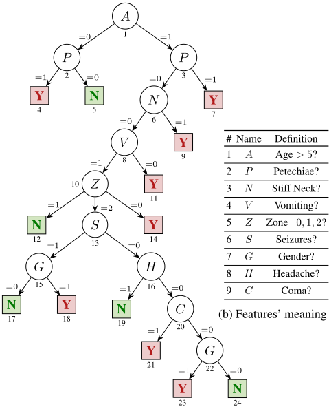
(a) Decision tree
Figure 1. A DT running example
single feature i ∈ F (i.e. univariate DTs), and the outgoing edges are associated with sets that partition the domain of i. Although in this paper we partition the domain of each feature by using literals of the form xi = di, in [Izza et al., 2022] we consider the more general setting where literals are of the form xi ∈ Ei, with Ei ⊆ Di. Moreover, each node of V is assigned a number (usually 1 is assigned to the root). Paths in the DT are represented as a sequence of numbers, e.g. P = 〈i1, i2, . . . , ir〉, such that each pair (ij, ij+1) denotes an edge of T . Furthermore, since each node partitions the domain of the feature, then no two paths can be consistent for the same point in feature space. In addition, for any path, it is assumed that there exists at least one point v in feature space for which the path's literals are consistent with v.
Running example. Throughout the paper, we will use the decision tree in Figure 1 [Lelis et al., 2020] as the running example. The DT serves to diagnose the most severe case of meningitis, Meningococcal Disease (MD), without invasive tests. Clearly, F = {1, . . . , 9}, K = {Y,N}, Di = {0, 1} for i = {1, 2, 3, 4, 6, 7, 8, 9}, and D5 = {0, 1, 2}. (Observe that Age is ordinal (integer or real), but we only test whether the value is greater than 5.) Moreover, we will consider the instance ((A = 1, P = 0,N = 0, V = 0,Z = 0, S = 0, H = 0, C = 0, G = 1), Y).
Logic-Based Explainability. We adopt a formal definition of explanation, as studied in recent works [Shih et al., 2018;
Ignatiev et al., 2019; Marques-Silva and Ignatiev, 2022; Marques-Silva, 2022].
Given an instance (v, c), an explanation problem E is a tuple (M, (v, c)). Moreover, a weak abductive explanation (WAXp) is a set of features X ⊆ F which, if assigned the values dictated by v, then the prediction is c. Formally,
(where the parametrization onMand (v, c) is shown.) Moreover, an abductive explanation (AXp) is a subset-minimal weak AXp:
WeakAXp(X) ∧ ∀(X ′ ⊊ X).¬WeakAXp(X ′ ) (2) (where the parametrization on M and (v, c) is not shown, and it is left implicit; we will do this henceforth.)
A weak contrastive explanation (WCXp) is a set of features Y ⊆ F which, if allowed to take any one of the values in their domain, then the prediction changes to a class other than c. Formally,
Moreover, a contrastive explanation (CXp) is a subsetminimal weak CXp:
Because the definitions of WAXp and WCXp are monotonic [Ignatiev et al., 2019; Marques-Silva and Ignatiev, 2022; Marques-Silva, 2022], then AXp's and CXp's can be computed more efficiently:
WeakCXp(Y) ∧ ∀(i ∈ Y).¬WeakCXp(Y \ {i}) (6) These latter definitions are at the core of algorithms for computing AXp's and CXp's. Finally, it is well-known that each AXp is a minimal hitting set (MHS) of the set of CXp's, and vice-versa [Ignatiev et al., 2020]. This MHS duality of AXp's and CXp's is at the core of algorithms for enumerating explanations.
Example 1. For the running example (see Figure 1), and the instance ((A = 1, P = 0,N = 0, V = 1,Z = 0, S = 0,H = 0,C = 0,G = 1),Y), we can show that one AXp is (A, Z) (technically, we should write (1, 5)). Thus, we can confidently state the following rule, representing a sufficient condition for predicting Y,
IF (Age > 5) ∧ (Zone = 0) THEN κ(·) =Y This conclusion is somewhat surprising, since we decide for the most severe case of meningitis, without actually requiring any symptoms to be observed. This example illustrates what seems to be an issue with the DT proposed in [Lelis et al., 2020]. In this case, the use of abductive explanations for DTs would allow uncovering the issue.
There has been rapid progress in logic-based explainability in recent years [Shih et al., 2018; Ignatiev et al., 2019; Darwiche and Hirth, 2020; Audemard et al., 2020; Barcel´o et al., 2020; Huang et al., 2021; Audemard et al., 2021; Izza and Marques-Silva, 2021; Ignatiev and Marques-Silva, 2021; Amgoud, 2021; Liu and Lorini, 2021; Huang et al., 2022; Ignatiev et al., 2022; Gorji and Rubin, 2022; Arenas et al., 2022]. Recent overviews include [Marques-Silva and Ignatiev, 2022; Marques-Silva, 2022].
3 Path Explanation Redundancy
For DTs, AXp's can either be restricted to a target path, i.e. the path consistent with the instance, or may include features from different paths. AXp's of the former kind are referred to as path-restricted, whereas AXp's of the latter kind are referred to as path-unrestricted. Path explanations are pathrestricted AXp's, with the additional property that no instance is specified; the path explanation applies to any instance consistent with the path. The identification of path-restricted AXp's reveals features which, if assigned one of its domain values tested in the path, is sufficient for the prediction. The remaining features are then deemed explanation redundant.
Path explanation redundancy in theory. The first main result is that the number of redundant features in a path can grow with the total number of features [Izza et al., 2022], which can be summarized as follows:
Proposition 1. There are DT classifiers, defined on m features, for which an instance has an AXp of size 1, and the consistent path has length m, and so it can be made larger by a factor of m than the size of an AXp.
The proof idea is to propose a classifier, and an optimal decision tree, such that there exists at least one path for which all literals but one are redundant. It turns out that this is fairly easy to do. Indeed, a boolean classifier that is the disjunction of the features will exhibit this extreme case of path explanation redundancy. Clearly, a possible criticism with respect Proposition 1 is that the proposed example classifier might be unique, or representative of a fairly restricted family of classifiers. In fact, the situation is exactly the opposite, and a DT will exhibit no path explanation redundancy only when the classifier being represented corresponds to the very restricted class of generalized decision functions (GDF) [Huang et al., 2022; Izza et al., 2022], concretely those that are binding, nonoverlapping and minimal (or irreducible). Thus, from [Izza et al., 2022, Proposition 11], we have:
Proposition 2. A DT T does not exhibit path explanation redundancy iff there exists a minimal DNF GDF g that is equivalent to T .
Overview of algorithms. We have devised different algorithms for computing AXp's, CXp's, and for their enumeration. This section briefly overviews these algorithms.
It is simple to find an AXp by iterated tree traversals. We pick an order of the features associated with the target path P with prediction c. This is the initial overapproximation of the AXp (and so a weak AXp); the remaining features not associated with the path are allowed to take any value from their domains, and so are excluded from the AXp. The features are analyzed in order. For each feature i, we allow i to take any value from its domain. We then traverse the tree, and if there is an assignment of values to the non-fixed features such that a path yielding a different prediction can be made consistent, then the feature cannot be allowed to take any value from its domain, and so it is fixed. Otherwise, if no path with a prediction other than c can be made consistent, then the feature is dropped from the set of features in the explanation. (A crucial observation is that the assumptions about decision trees guarantee that for any path, some point v in feature space is consistent with the path; hence checking consistency runs in polynomial time on the size of the path.)
In practice, an approach that is more efficient than iterated tree traversals is to encode the problem as a propositional Horn formula, containing both hard and soft clauses, such that the soft clauses capture a preference not to pick features, i.e. a partial (Horn) MaxSAT (i.e. a smallest maximal satisfiable subset (MSS)) encoding. Finding an optimal solution for partial (Horn) MaxSAT is NP-hard. However, finding an MSS (and so indirectly an AXp) is polynomial-time solvable in the size of the DT [Izza et al., 2022].
To change the prediction, we can pick any path Q with a prediction other than c, traverse the path Q and, for the features in Q that are fixed (given P) and are inconsistent with the value(s) dictated by P, then we add them to the set features in the CXp. (A technical detail is that we need to check that no other path with prediction other that c will allow for a strictly smaller subset of features. Since the number of paths is polynomial on the tree size, then the algorithm runs in polynomial time.
The same algorithm that is used for computing one CXp can be modified for enumerating all the CXp's. Clearly, each path Q with a prediction other than c can represent at most one CXp (and there can exist paths that do not contribute any CXp B because some other path contributes a CXp A that is a proper subset of B). Hence, enumeration of CXp's is polynomial-time solvable in the case of DTs [Huang et al., 2021; Izza et al., 2022].
The next examples illustrate the (simpler) algorithms developed for explaining DTs.
Example 2 (Computation of one AXp). For the running example of Figure 1, consider the path P = 〈1, 3, 6, 8, 10, 14〉, with prediction Y. The set of features of interest is {A, P,N, V,Z}; the remaining features we will discard for path-restricted AXp's. It is immediate to conclude that, by allowing P,N, V to take any value from their domain, the prediction remains at Y. By inspection, allowing any of the remaining features to take any value from its domain will allow the prediction to change. Hence, the AXp is {A,Z} (or using feature numbers, {1, 5}.) As can be readily concluded, the AXp contains 2 (out of 9) features; hence the fraction of redundant features is 77.8%.
Example 3 (Computation of one CXp). For the same path P above, we consider the path Q = 〈1, 2, 5〉. Clearly, P takes the same value in the two paths, and so it is discarded. Finally, we can make the path Q consistent by setting A = 0. Hence, one CXp is {A} (or {1}). To find the second CXp, we can consider the path R = {1, 3, 6, 8, 10, 12}. In this case, the only feature that takes a value different from the values of the literals in P is Z. Hence, by changing the value of Z from 0 to 1, we force the prediction to change. Hence, the other CXp is {Z} (or {5}). (This is to be expected by minimal hitting set duality [Ignatiev et al., 2020].)
3.1 Path Explanation Redundancy in Practice
In practice, the experiments in [Izza et al., 2022] confirm the theoretical results. First, the vast majority of DTs, generated with a wide range of decision tree learning algorithms (including algorithms that learn optimal decision trees), exhibit path explanation redundancy. As shown in Section 4, path explanation redundancy is significant, both in terms of the number of paths that are explanation redundant, but also in terms of the number of literals that are redundant in any given path. Moreover, [Izza et al., 2022] also shows that path explanation redundancy is ubiquitous in example DT used in papers and books since the early 80s. The next section overviews the experimental results from [Izza et al., 2022].
4 Experimental Evidence
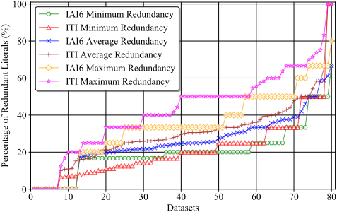
[Izza et al., 2022] presents a wide range of results, covering example DTs found in many publications since the early 80s, to DTs learned with different tree-learning algorithms, some of which learn optimal DTs. This section summarizes the experimental results in [Izza et al., 2022], but also includes more recent data points. Figure 2 aggregates the redundancy results obtained with well-known (optimal) tree-learning algorithms, namely the tool from Interpretable AI [Bertsimas and Dunn, 2017] and ITI [Utgoff et al., 1997]. As can be observed, for most DTs, path explanation redundancy can be observed, and the fraction of redundant paths can reach close to 100%. Table 1 sumarize path-explanation redundancy for four well-known datasets, using two optimal tree-learning tools, namely BinOCT [Verwer and Zhang, 2019] and OSDT/GOST [Hu et al., 2019; Lin et al., 2020]. The results for CART [Breiman et al., 1984] are included for completeness. As claimed earlier, optimal DTs can exhibit path explanation redundancy.
The experiments reported in this work consider fairly shallow DTs (i.e. with depths not exceeding most often 6 or 8). The sole reason for using shallow trees is that these suffice in terms of target accuracy, i.e. deeper trees do not yield improvements in accuracy. However, the methods proposed in this work can be shown to apply to much larger (and deeper) DTs. For example, recent work [Ghiasi et al., 2020] proposes the use of DTs for diagnosis of coronary artery disease. For one of the DTs proposed in [Ghiasi et al., 2020] (see [Ghiasi et al., 2020, Fig. 2]) the longest paths have 19 non-terminal nodes. Among these, for the path with prediction CAD, manual inspection 1 reveals that at least 10 literals out of 19 (i.e. more than 50%) are redundant. Evidently, for a human decision maker, an explanation with 9 literals (or less) is far easier to understand than one with 19 literals. Manual inspection of the additional DTs reported in [Ghiasi et al., 2020] confirm that these exhibit a similar degree of redundancy.
| Dataset | Tool | D | #N | %A | #P | %R | %C | %m | %M | %avg |
|---|---|---|---|---|---|---|---|---|---|---|
| monk1 | BinOCT OSDT | 3 5 | 13 13 | 91 100 | 7 7 | 28 57 | 11 41 | 66 33 | 66 33 | 66 33 |
| tic-tac-toe | BinOCT OSDT | 4 5 | 15 15 | 77 83 | 8 8 | 75 75 | 75 37 | 33 25 | 33 60 | 33 43 |
| compas | OSDT | 4 | 9 | 67 | 5 | 60 | 37 | 33 | 33 | 33 |
| monk2 | CART GOSDT | 6 6 | 31 17 | 69 73 | 16 9 | 62 55 | 22 48 | 20 16 | 66 40 | 33 31 |
5 Conclusions
One established misconception in explainability/interpretability is that decision trees (and other so-called interpretable models) are intrinsically interpretable, i.e. the ML model yields itself explanations for predictions [Rudin, 2019; Molnar, 2020]. Our work [Izza et al., 2022] disproves this misconception. We have shown that DTs can exhibit path explanation redundancy, i.e. features in paths that are unnecessary for the prediction, and that such redundancy can be arbitrarily large on the number of features. We have also proved that the subclass of DTs that do not exhibit explanation redundancy is fairly restricted. Besides the theoretical results, we have demonstrated that a vast number of DTs, which have been used in publications since the early 80s (i.e. since the inception of DT learning algorithms), exhibit explanation redundancy, and that such explanation redundancy can be significant. Finally, we have also shown that algorithms for learning DTs, either optimal or non-optimal, exhibit explanation redundancy.
The results of our work are clear, and decision trees (and other interpretable models) should be explained in practice. Moreover, it would be important to learn decision trees representing functions that offer simple explanations instead of learning decision trees that target some other metric, e.g. tree depth or tree size. This is the subject of future research.
1 Unfortunately, we have been unable to obtain from the authors this concrete DT in a format suitable for automated analysis.
@inproceedings{ijcai2023p779,
  title     = {On Tackling Explanation Redundancy in Decision Trees (Extended Abstract)},
  author    = {Izza, Yacine and Ignatiev, Alexey and Marques-Silva, Joao},
  booktitle = {Proceedings of the Thirty-Second International Joint Conference on
               Artificial Intelligence, {IJCAI-23}},
  publisher = {International Joint Conferences on Artificial Intelligence Organization},
  editor    = {Edith Elkind},
  pages     = {6900--6904},
  year      = {2023},
  month     = {8},
  note      = {Journal Track},
  doi       = {10.24963/ijcai.2023/779},
  url       = {https://doi.org/10.24963/ijcai.2023/779},
}
TY - CPAPER TI - On Tackling Explanation Redundancy in Decision Trees (Extended Abstract) AU - Izza, Yacine AU - Ignatiev, Alexey AU - Marques-Silva, Joao T2 - Proceedings of the Thirty-Second International Joint Conference on Artificial Intelligence, IJCAI-23 PB - International Joint Conferences on Artificial Intelligence Organization PY - 2023 SP - 6900 EP - 6904 DO - 10.24963/ijcai.2023/779 UR - https://doi.org/10.24963/ijcai.2023/779 ER -Copied
Machine-readable versions of this paper, for tools and AI agents:





