
Multi-objective Search via Lazy and Efficient Dominance Checks
Proceedings of the Thirty-Second International Joint Conference on Artificial Intelligence. Main Track. Pages 7223-7230.
https://doi.org/10.24963/ijcai.2023/850
Keywords
- Search: S: Heuristic search
- Robotics: ROB: Motion and path planning
- Search: S: Combinatorial search and optimisation
Abstract
Multi-objective search can be used to model many real-world problems that require finding Pareto optimal paths from a specified start state to a specified goal state, while considering different costmetrics such as distance, time, and fuel. The performance of multi-objective search can be improved by making dominance checking—an operation necessary to determine whether or not a path dominates another—more efficient. This was shown in practice by BOA*, a state-of-the-art bi-objective search algorithm, which outperforms previously existing bi-objective search algorithms in part because it adopts a lazy approach towards dominance checking. EMOA*, a recent multi-objective search algorithm, generalizes BOA* to more-than-two objectives using AVL trees for dominance checking.
In this paper, we first propose Linear-Time Multi-Objective A* (LTMOA*), an multi-objective search algorithm that implements a more efficient dominance checking than EMOA* using simple data structures like arrays. We then propose an even lazier approach towards dominance checking, and the resulting algorithm, LazyLTMOA*, distinguishes from EMOA* and LTMOA* by removing the dominance checking during node generation. Our experimental results show that LazyLTMOA* outperforms EMOA* by up to an order of magnitude in terms of runtime.
- [Ahmadi et al., 2021] Saman Ahmadi, Guido Tack, Daniel Harabor, and Philip Kilby. Bi-objective search with bi- directional A*. In Proceedings of the European Sympo- sium on Algorithms, volume 204, pages 3:1-3:15, 2021.
- [Bachmann et al., 2018] Daniel Bachmann, Fritz Bökler, Jakob Kopec, Kira Popp, Björn Schwarze, and Frank We- ichert. Multi-objective optimisation based planning of power-line grid expansions. ISPRS International Journal of Geo-Information, 7(7):258, 2018.
- [Bronfman et al., 2015] Andrés Bronfman, Vladimir Mari- anov, Germán Paredes-Belmar, and Armin Lüer-Villagra. The maximin hazmat routing problem. European Journal of Operational Research, 241(1):15-27, 2015.
- [Casas et al., 2021] Pedro Maristany de las Casas, Luitgard Kraus, Antonio Sedeño-Noda, and Ralf Borndörfer. Tar- geted multiobjective dijkstra algorithm. arXiv preprint arXiv:2110.10978, 2021.
- [Fu et al., 2019] Mengyu Fu, Alan Kuntz, Oren Salzman, and Ron Alterovitz. Toward asymptotically-optimal in- spection planning via efficient near-optimal graph search. In Proceedings of Robotics: Science and Systems, 2019.
- [Fu et al., 2021] Mengyu Fu, Oren Salzman, and Ron Al- terovitz. Computationally-efficient roadmap-based inspec- tion planning via incremental lazy search. In Proceedings of International Conference on Robotics and Automation, pages 7449-7456, 2021.
- [Hernández et al., 2023] Carlos Hernández, William Yeoh, Jorge A. Baier, Han Zhang, Luis Suazo, Sven Koenig, and Oren Salzman. Simple and efficient bi-objective search algorithms via fast dominance checks. Artificial Intelli- gence, 314:103807, 2023.
- [Li et al., 2015] B. Li, J. Li, K. Tang, and X. Yao. Many- objective evolutionary algorithms: A survey. ACM Com- puting Surveys, 48(1):1-35, 2015.
- [Mandow and De La Cruz, 2010] Lawrence Mandow and José Luis Pérez De La Cruz. Multiobjective A* search with consistent heuristics. Journal of the ACM, 57(5):27:1-27:25, 2010.
- [Mandow et al., 2005] Lawrence Mandow, JL Pérez De la Cruz, et al. A new approach to multiobjective A* search. In Proceedings of International Joint Conference of Artifi- cial Intelligence, pages 218-223, 2005. IJCAI
- [Pangilinan and Janssens, 2007] J. M. Pangilinan and G. Janssens. Evolutionary algorithms for the multiobjec- tive shortest path problem. World Academy of Science, Engineering and Technology, 25:205-210, 2007.
- [Pulido et al., 2015] Francisco-Javier Pulido, Lawrence Mandow, and José-Luis Pérez-de-la-Cruz. Dimension- ality reduction in multiobjective shortest path search. Computers & Operations Research, 64:60-70, 2015.
- [Ren et al., 2022] Zhongqiang Ren, Richard Zhan, Sivaku- mar Rathinam, Maxim Likhachev, and Howie Choset. En- hanced multi-objective a* using balanced binary search trees. In Proceedings of the International Symposium on Combinatorial Search, pages 162-170, 2022.
- [Salzman and Goldin, 2021] Oren Salzman and Boris Goldin. Approximate bi-criteria search by efficient representation of subsets of the Pareto-optimal fron- tier. In Proceedings of the International Conference on Automated Planning and Scheduling, pages 149-158, 2021.
- [Skyler et al., 2022] S. Skyler, D. Atzmon, A. Felner, O. Salzman, H. Zhang, S. Koenig, W. Yeoh, and C. Hernández. Bounded-cost bi-objective heuristic search. In Proceedings of the International Symposium on Combi- natorial Search, pages 239-243, 2022.
- [Zhang et al., 2022a] H. Zhang, O. Salzman, T. K. S. Kumar, A. Felner, C. Hernández, and S. Koenig. Anytime approx- imate bi-objective search. In Proceedings of the Interna- tional Symposium on Combinatorial Search, pages 199- 207, 2022.
- [Zhang et al., 2022b] H. Zhang, O. Salzman, TK S. Kumar, A. Felner, C. Hernández, and S. Koenig. A*pex: Efficient approximate multi-objective search on graphs. In Proceed- ings of the International Conference on Automated Plan- ning and Scheduling, pages 394-403, 2022.
References were extracted automatically from the PDF and may contain errors.
Full text extracted automatically from the PDF; figures, tables and equations may differ. The PDF is the version of record.
1 Introduction and RelatedWork
Multi-objective search can be used to model many real-world problems that involve planning paths with more than one cost metric, such as distance, time, and fuel. Each objective corresponds to minimizing a specific cost metric. Examples of such real-world problems include planning of powerline routes in energy transmission domains [Bachmann et al., 2018], balancing travel distance and risk of exposure when transporting a hazardous material [Bronfman et al., 2015], and inspecting a region of interest using cameras placed onboard robotic platforms [Fu et al., 2019; Fu et al., 2021]. While single-objective search produces shortest paths with respect to a single cost metric, it needs to be efficiently generalized to multi-objective search for the aforementioned real-world problems. Generally, the desired output of multiobjective search is a set of non-dominated paths with respect to the different cost metrics.
More formally, in multi-objective search, we are given a directed graph with multiple costs annotating each edge, a specified start state, and a specified goal state. A path π is considered to be better than, i.e., to dominate, another path π′ if and only if π is not worse than π′ on any cost metric and π is better than π′ on at least one cost metric, and a Paretooptimal solution is a path from the start state to the goal state that are not dominated by any path from the start state to the goal state. We are interested in computing the Pareto-optimal solution set, that is, the set of all Pareto-optimal solutions.
Importantly, different variants of the problem exist such as approximating the Pareto-optimal solution set [Salzman and Goldin, 2021; Zhang et al., 2022b; Pangilinan and Janssens, 2007; Li et al., 2015] and computing the Pareto-optimal solution set in an anytime manner [Zhang et al., 2022a]. Researchers have also computed a single solution in the Paretooptimal solution set given bounds on its cost [Skyler et al., 2022] and using bi-directional search [Ahmadi et al., 2021]. However, these are out of the scope of the paper.
Existing algorithms for computing the Pareto-optimal solution set include NAMOA* [Mandow et al., 2005; Mandow and De La Cruz, 2010], NAMOA* with dimensionality reduction (NAMOA*dr) [Pulido et al., 2015], Enhanced MultiObjective A* (EMOA*) [Ren et al., 2022], and Bi-Objective A* (BOA*) [Hern´andez et al., 2023]. All of these algorithms perform dominance checks to determine if a path from the start state to a specific state has the potential to be extended to a Pareto-optimal solution. However, they differ in how the dominance checks are implemented and interleaved with the search. Both NAMOA* and NAMOA*dr can be used for any number of objectives and perform dominance checks eagerly: Every time they generate a path to a specific state, they eagerly check if this path is dominated by any previously generated path to the same state, which involves time-consuming operations that iterate over generated paths. BOA* shows that some of these time-consuming operations can be alleviated using a lazy approach for dominance checks and performs all dominance checks in constant time by doing so. However, it is restricted to solving problems with only two objectives. The recently proposed EMOA* algorithm generalizes the lazy dominance checks of BOA* to more than two objective. For problems with three objectives, it uses AVL trees and performs dominance checks in logarithmic time when generating a path.
In this paper, we first investigate different data structures that can be used for dominance checks and propose Linear-Time Multi-Objective A* (LTMOA*), an multiobjective search algorithm that implements a more efficient dominance checking than EMOA* using simple data structures like arrays. We then propose an even "lazier" approach towards dominance checking than those of EMOA* and LTMOA*. The resulting algorithm, LazyLTMOA*, distinguishes from EMOA* and LTMOA* by removing dominance checking during node generation and only performing dominance checking when a path is selected for expanding.
We evaluate LTMOA* and LazyLTMOA* on road network instances with up to five objectives. Empirically, we show that LazyLTMOA* is about 60% faster than LTMOA* due to less dominance checking. With our efficient dominance checking approach, LazyLTMOA* substantially outperforms EMOA* by up to an order of magnitude in terms of runtime.
2 Notation and ProblemDefinition
A multi-objective search graph is a tuple (S, E, c), where S is the finite set of states, E ⊆ S ×S is the finite set of edges, and c : E → (R≥0)n is a cost function that associates an n-tuple of non-negative real costs with each edge, where n is the number of components. Succ(s) = {t ∈ S | (s, t) ∈ E} denotes the successors of state s. A path π from s1 to sm is a sequence of states s1, s2, . . . , sm such that (si, si+1) ∈ E for all i ∈ {1, . . . ,m-1}.
Boldface font is used to represent n-tuples. Unless defined otherwise, we assume a n-tuple v has the form v = (v1, v2, . . . , vn), thus vi denotes the i-th component of an ntuple. The addition of two n-tuples u and v and the multiplication of a real-valued scalar k and a tuple u are defined in the natural way; that is, u+v = (u1 +v1, . . . , un +vn) and ku = (ku1, . . . , kun). c(π) = ∑m-1 i=1 c(si, si+1) is the cost of path π = s1, . . . , sm.
Given two n-tuples u and v, we say that u weakly dominates v, denoted as u ⪯ v, if vi ≤ ui holds for every i ∈ {1, . . . , n}. We say u dominates v, denoted as u ≺ v, if u ⪯ v and u ̸= v hold. We say that path π dominates (resp. weakly dominates) path π′ , denoted as π ≺ π′ (resp. π ⪯ π′ ) if c(π) ≺ c(π′ ) (resp. c(π) ⪯ c(π′ )).
A search instance is defined as a tuple P = (S,E, c, sstart, sgoal), where (S,E, c) is a search graph and sstart, sgoal ∈ S are the start and goal states, respectively. Given a search instance P, a Pareto-optimal solution set to sgoal (from sstart), denoted as sols(sgoal), contains every path π from sstart to sgoal with the property that, for every other path π′ from sstart to sgoal, π′ ̸≺ π holds; that is, sols(sgoal) contains all non-dominated paths from sstart to sgoal. In this paper, we aim to find any maximal subset of the Pareto-optimal solution set such that each solution in the subset has a unique
Algorithm 1: NAMOA*
Input : A search problem (S,E, c, sstart, sgoal) and a consistent heuristic function h Output: A cost-unique Pareto-optimal solution set 1 sols ← ∅ 2 for each s ∈ S do 3 Gop(s) ← ∅; Gcl(s) ← ∅ 4 x ← new node with s(x) = sstart 5 g(x) ←zero in all dimensions 6 Add g(x) toGop(s(x)) 7 p(x) ←null 8 f(x) ←h(sstart) 9 Initialize Open and add x to it 10 while Open ̸= ∅ do 11 Extract a node x from Open with the lexicographically smallest f-value 12 Remove g(x) fromGop(s(x)) 13 if IsDominated(f(x), Gcl(sgoal)) then 14 continue 15 Add g(x) toGcl(s(x)) 16 if s(x) = sgoal then 17 Add x to sols 18 continue 19 for each t ∈ Succ(s(x)) do 20 x′ ← new node with s(x′ ) = t 21 g(x′ ) ← g(x) + c(s(x), t) 22 p(x) ← x 23 f (x′ ) ← g(x′ ) + h(t) 24 if IsDominated(g(x′ ),Gcl(t) ∪Gop(t)) or IsDominated(f(x′ ),Gcl(sgoal)) then 25 continue 26 UpdateOpen(x′ )27 return sols
Algorithm 2: IsDominated
Input : A vector v and a set of vector V Output: true or false 1 for each v′ ∈ V do 2 if v′ ⪯ v then 3 return true 4 return falsecost of path. We refer to this subset as a cost-unique Paretooptimal solution set.
A heuristic function h maps each state s in S to a n-tuple in (R≥0)n domain that estimates the cost of a path from state s to sgoal. Given a heuristic function h, the h-value of state s is denoted as h(s). h is admissible iff h(s) ⪯ c(π) holds for every state s and every path π that traverses s from sstart to sgoal. Similarly, h is consistent iff (i) h(sgoal) = 0 and (ii) h(s) ⪯ c(s, t) + h(t) for every (s, t) ∈ E. That is, all components of h are consistent for the corresponding components of the cost function.
3 Algorithmic Background
We now describe the multi-objective search algorithms that form the building blocks for our new algorithm. All algorithms perform a best-first search and compute a cost-unique Pareto-optimal solution set for a given search instance. Thus, we start with general notations and assumptions that will be used for all algorithms (including our own) and then describe each algorithm while highlighting the differences. All the al-
Input : A node x Output: Open and Gop(s(x)) updated 1 for each g′ ∈ Gop(s(x)) do 2 if g(x) ⪯ g′ then 3 Remove g′ fromGop(s(x)) 4 Remove nodes corresponding to g′ fromOpen 5 Add g(x) toGop(s(x)) 6 Add x to OpenAlgorithm 3: UpdateOpen 7 returngorithms maintain an Open list, containing the frontier of the search tree (i.e., the generated but not-yet-expanded nodes) and a set of solutions sols. Here, a node x is associated with a state s(x) ∈ S, a g-value g(x), and a parent node p(x). We also define f(x) = g(x) + h(s(x)) as the f-value of x. Conceptually, x corresponds to a path from sstart to s(x) with cost g(x). The path can be constructed by backtracking along the parent nodes. We assume that the reader is familiar with the properties of A* when used with consistent h-values, for example, that the sequence of expanded nodes has monotonically non-decreasing f -values.
NAMOA*: For any state s, NAMOA* (Algorithm 1) maintains two sets of g-values, Gcl(s) and Gop(s). 1 These sets store the non-dominated g-values for all the expanded nodes and for all the generated but not-yet-expanded nodes associated with state s, respectively. These two sets are used to perform dominance checks in order to prune nodes that cannot be part of the Pareto-optimal set. To check if a given n-tuple v is dominated by a n-tuple in a given set of n-tuples V, the algorithm iterates through V, which takes linear time in |V|, as shown in Algorithm 2.
In each iteration, NAMOA* extracts a node x from Open whose f-value is not dominated by the f-value of any node in Open. One way to select such a non-dominated node is to select a node with the lexicographically smallest f-value (Line 11). Node x is pruned if f (x) is dominated by a g-value in Gcl(sgoal) (Lines 13-14). Otherwise, NAMOA* adds g(x) to Gcl(s(x)) (Line 15) and expands x. If state s(x) is the goal state sgoal, then NAMOA* adds (the corresponding path of) x to sols (Lines 16-18). Otherwise, it generates a child node x′ for each successor t of state s(x). Node x′ is pruned if its g-value is dominated by a g-value in Gcl(t) ∪ Gop(t) or if its f -value is dominated by a g-value in Gcl(sgoal) (Lines 2425). If node x′ is not pruned, then NAMOA* removes all nodes with state t and whose g-values are dominated by g(x′ ) from Open and their g-values from Gop(t), and adds node x′ to Open and its g-value to Gop(s(x′ )) (see Algorithm 3).
NAMOA*dr: Recall that each dominance check performed by NAMOA* (Lines 13 and 24, Algorithm 1) requires a lineartime iteration over Gcl(s) and Gop(s) for each state s considered. This operation is time-consuming and can often dominate the algorithm's runtime. NAMOA*dr [Pulido et al., 2015] improves the processes by using a technique called dimensionality reduction to reduce the size of Gcl and thus reduce the time taken to perform dominance checks subsequently.
1 'cl' and 'op' are shorthand for 'closed' and 'open', respectively.
NAMOA*dr uses a consistent heuristic and extracts a node with the lexicographically smallest f-value among all nodes in Open in each iteration. Thus, when NAMOA*dr extracts or generates a node x, we always have that g1(x) ≥ max{g1 | g ∈ Gcl(s(x))} and that f1(x) ≥ max{g1 | g ∈ Gcl(sgoal)}. Therefore, there is no need to consider the first component of g- or f in dominance checks. To this end, let the truncated vector of a vector v with length n, denoted as Tr(v), be the vector consisting of its last n - 1 elements. That is, Tr(v) = (v2, . . . , vn). For a state s, NAMOA*dr only needs to maintain the set of non-dominated truncated g-values for all expanded nodes, namely GTr cl (s), which is often significantly smaller than the size of Gcl(s) [Pulido et al., 2015]. As the gvalues of generated nodes are not necessarily monotonically and lexicographically increasing, to check whether a generated node x is dominated by some node in Open associated with state s(x), NAMOA*dr still needs to completely iterate over Gop(s(x)).
BOA*: BOA* [Hern´andez et al., 2023] is a bi-objective (that is, with exactly two objectives) search algorithm which also builds upon the dimensionality reduction technique of NAMOA*dr. In the specific setting of bi-objective search, the truncated g-value is a single number g2 (2 is the index of the 2nd and last dimension), and a non-dominated truncated g-value set can be represented by the minimum g2-value of all g-values. For all expanded nodes associated with some state s, BOA* stores this minimum value in gmin 2 (s). When a node x is extracted from Open or generated, BOA* prunes node x if f (x) ≥ gmin 2 (sgoal) or if g(x) ≥ gmin 2 (s(x)) holds.
BOA* and NAMOA*dr differ in the way dominance checks are performed. BOA* performs a dominance check for a node x (both when generating it and when extracting it from Open) by matching x against gmin 2 (s(x)) (which is equivalent to performing dominance check in Closed). But when x is generated, BOA* does not check if the node is dominated by some node in Open. Therefore, the greatest advantage of BOA* is that all dominance checks of BOA* are done in constant time (against gmin 2 ). But since no pruning is done with nodes in Open, there is a risk in BOA* of having a larger Open compared to NAMOA*dr. Nevertheless, Hern´andez et al. [2023] showed empirically that BOA* significantly outperforms both NAMOA* and NAMOA*dr in terms of runtime (due to the much smaller dominance check overhead) on a wide suite of benchmarks of road network instances.
Multi-Objective Search Framework and EMOA*: Recently, Ren et al. [2022] proposed a Multi-Objective Search Framework (MOSF) that generalizes BOA* to more than two objectives. Similar to BOA*, when a node x is generated, a particular algorithm in MOSF performs dominance checks against only Gcl(s(x)) and Gcl(sgoal) while ignoring Open. The EMOA* [Ren et al., 2022] algorithm is a particular case of MOSF. EMOA* also utilizes the dimensionality reduction technique. It extracts nodes in the increasing lexicographic order and maintains the set of non-dominated truncated gvalues GTr cl (s) for each state s. Specifically, EMOA* uses an AVL tree to store GTr cl (s) for each state s. With three objectives, the dominance check against GTr cl (s) takes in logarithmic time in terms of the number of elements in GTr cl (s),
Algorithm 4: RemoveDominated
Input : A vector v and a set of vectors V Output: V updated 1 for each v′ ∈ V do 2 if v ⪯ v′ then 3 Remove v′ fromV 4 returnAlgorithm 5: LTMOA*
Input : A search problem (S,E, c, sstart, sgoal) and a consistent heuristic function h Output: A cost-unique Pareto-optimal solution set 1 sols ← ∅ 2 for each s ∈ S do 3 GTr cl (s) ← ∅ 4 x ← new node with s(x) = sstart 5 g(x) ←zero in all dimensions 6 p(x) ←null 7 f(x) ←h(sstart) 8 Initialize Open and add x to it 9 while Open ̸= ∅ do 10 Extract a node x from Open with the lexicographically smallest f-value 11 if IsDominated(Tr(g(x)), GTr cl (s(x))) or IsDominated(Tr(f (x)), GTr cl (sgoal)) then 12 continue 13 RemoveDominated(Tr(g(x)), GTr cl (s(x))) 14 Add gT(x) toGTr cl (s(x)) 15 if s(x) = sgoal then 16 Add x to sols 17 continue 18 for each t ∈ Succ(s(x)) do 19 y ← new node with s(y) = t 20 g(y) ← g(x) + c(s(x), t) 21 p(y) ← x 22 f (y) ← g(y) + h(t) 23 if IsDominated(Tr(g(y)),GTr cl (t)) or IsDominated(Tr(f (y)), GTr cl (sgoal)) then 24 continue 25 Add y to Open 26 return solsdenoted as |GTr cl (s)|. However, with more than three objectives, EMOA*'s dominance checks still takes linear time on |GTr cl (s)|. Ren et al. [2022] showed empirically that EMOA* outperforms NAMOA*dr in terms of runtime on road network instances with three objectives.
4 LTMOA*
In this section, we describe Linear Time MOA* (LTMOA*), a new particular case of MOSF that performs dominance check in linear time using a linked list or an array to store GTr cl (s) for each state s. Algorithm 5 shows the pseudocode for LTMOA*. LTMOA* maintains GTr cl (s), a set of nondominated truncated g-values for each state s. In contrast to NAMOA* and NAMOA*dr, LTMOA* does not maintain Gop(s). When extracting or generating a node x, LTMOA* prunes x if (i) Tr(f(x)) is weakly dominated by any vectors in GTr cl (sgoal); or if (ii) Tr(g(x)) is weakly dominated by any vector in GTr cl (s(x)) (Lines 11 and 23). Similar to BOA*, LTMOA* does not check if a generated node is dominated by nodes in Open associated with the same state. Thus, multiple copies of the same state (one dominating the other) may be simultaneously in Open. Then, after choosing node x for expansion, LTMOA* removes all (truncated) g-values that are dominated by Tr(g(x)) from GTr cl (s(x)) (Line 13) and then inserts Tr(g(x)) to GTr cl (s(x)) (Line 14).
| Iter | Open ⟨s(x), g(x), f(x)⟩ | Update of GTr cl (s(x)) |
|---|---|---|
| 1 | ⟨sstart, (0, 0, 0), (2, 3, 3)⟩∗ | GTr cl (sstart) = {(0, 0)} |
| 2 | ⟨s1, (1, 1, 1), (2, 3, 5)⟩∗ ⟨s2, (1, 3, 2), (2, 4, 3)⟩ | GTr cl (s1) = {(1, 1)} |
| 3 | ⟨s2, (1, 3, 2), (2, 4, 3)⟩∗ ⟨s2, (4, 2, 4), (5, 3, 5)⟩ ⟨sgoal , (2, 4, 5), (2, 4, 5)⟩ | GTr cl (s2) = {(3, 2)} |
| 4 | ⟨sgoal , (2, 4, 3), (2, 4, 3)⟩∗ ⟨s2, (4, 2, 4), (5, 3, 5)⟩ ⟨sgoal , (2, 4, 5), (2, 4, 5)⟩ | GTr cl (sgoal) = {(4, 3)} |
| 5 | ⟨s2, (4, 2, 4), (5, 3, 5)⟩ ⟨sgoal , (2, 4, 5), (2, 4, 5)⟩∗ | |
| 6 | ⟨s2, (4, 2, 4), (5, 3, 5)⟩∗ | GTr cl (s2) = {(3, 2), (2, 4)} GTr cl (sgoal) = {(4, 3), (3, 5)} |
| 7 | ⟨sgoal, (5, 3, 5), (5, 3, 5)⟩∗ | |
| 8 | empty |
In Algorithm 5, we highlight some differences of LTMOA* compared to NAMOA*dr in blue. When generating a node x, NAMOA*dr performs more dominance checks than LTMOA* as it needs to iterate over Gop(s(x)). More specifically, assuming that x is not pruned, NAMOA*dr iterates over Gop(s(x)) twice: It first checks if g(x) is dominated by any g-value in Gop(s(x)) (Line 24, Algorithm 1), and then it needs to check if each g-value in Gop(s(x)) should be removed. In contrast, LTMOA* does not perform the dominance checks with Gop(s(x)) but, instead, performs more dominance checks when it extracts x for expansion.
The main difference between LTMOA* and EMOA* is how dominance checks are implemented. In EMOA* the dominance checks are implemented with AVL trees. We provide two other approaches for dominance checks, which use different data structures than AVL trees: (1) Linked List: For each state s, GTr cl (s) is stored as a linked list. Both IsDominated and RemoveDominated iterate through the entire linked list and hence take linear time of |GTr cl (s)|. (2) Array: For each state s, GTr cl (s) is stored as an array. When removing a g-value from GTr cl (s), LTMOA* first swap this g-value with the last gvalue in the array and then pop the last g-value from the array, which takes only constant time.
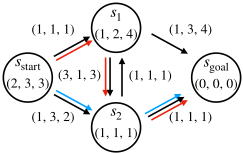
Figure 1 shows a toy problem instance with three objectives with Pareto-optimal paths in this problem instance:
sstart, s2, sgoal (shown by blue arrows) with cost (2, 4, 3) and sstart, s1, s2, sgoal (shown by red arrows) with cost (5, 3, 5). Table 1 shows a trace of Open and changes to GTr cl in each iteration of LTMOA*. In Iterations 1-2, LTMOA* expands nodes ⟨sstart, (0, 0, 0), (2, 3, 3)⟩ and ⟨s1, (1, 1, 1), (2, 3, 5)⟩, and then generates node ⟨sgoal, (2, 4, 5), (2, 4, 5)⟩, which is associated with sgoal. However, in Iterations 3-4, LTMOA* finds a solution with cost (2, 4, 3). Hence, node ⟨sgoal, (2, 4, 5), (2, 4, 5)⟩ is extracted and pruned in Iteration 5. In Iteration 3, node ⟨s1, (2, 4, 3), (3, 6, 7)⟩ is also generated when expanding node ⟨s2, (1, 3, 2), (2, 4, 3)⟩. However, it is not added to Open since it is pruned (and hence not shown in the table) as Tr(2, 4, 3) = (4, 3) is dominated by (1, 1) ∈ GTr cl (s1). In Iteration 6, the node associated with s1, generated when expanding node ⟨s2, (4, 2, 4), (5, 3, 5)⟩ is also pruned.
If we use NAMOA*dr to solve this problem instance, node ⟨sgoal, (2, 4, 5), (2, 4, 5)⟩ will be removed from Open in Iteration 3 when node ⟨sgoal, (2, 4, 3), (2, 4, 3)⟩ is inserted to Open, and the algorithm will terminate in Iteration 7. Despite having fewer iterations, NAMOA*dr needs to perform more dominance checks: In Iteration 2, when generating node ⟨s2, (4, 2, 4), (5, 3, 5)⟩, NAMOA*dr needs to check if its g-value (4, 2, 4) and (1, 3, 2), that is, the g-value in Gop(s2), dominates each other. Meanwhile LTMOA* inserts node ⟨s2, (4, 2, 4), (5, 2, 5)⟩ into Open without performing such dominance checks, and it only needs to perform one additional dominance check between (2, 4) and (3, 2) in Iteration 6 before expanding the node.
5 A LazyMulti-Objective Search Framework
We propose an even "lazier" framework in terms of dominance checks, Lazy MOSF, which is a simple extension of MOSF where dominance checks during node generation is totally removed. To explain how the framework works, we describe LazyLTMOA*, a Lazy-MOSF variant of LTMOA*. While LTMOA* performs dominance checks against truncated g-values of expanded nodes when a node is generated or extracted from Open, LazyLTMOA* performs dominance checks only when a node is extracted from Open (line 11 of Algorithm 5). We omit the pseudo code for LazyLTMOA* since if can be obtained by removing Lines 23-24 from Algorithm 5.
Consider LazyLTMOA* and the problem instance in Figure 1. Table 2 shows a trace of Open and changes to GTr cl in each iteration of LazyLTMOA*. In Iteration 3, node ⟨s1, (2, 4, 3), (3, 6, 7)⟩ is generated by LazyLTMOA* when expanding ⟨s2, (1, 3, 2), (2, 4, 3)⟩ and inserted into Open (whereas LTMOA* prunes ⟨s1, (2, 4, 3), (3, 6, 7)⟩). Later, in Iteration 6, node ⟨s1, (2, 4, 3), (3, 6, 7)⟩ is extracted from Open and then pruned. Similarly, in Iteration 7, node ⟨s1, (5, 3, 5), (6, 5, 9)⟩ is also generated and inserted into Open when expanding ⟨s2, (4, 2, 4), (5, 3, 5)⟩. Although LazyLTMOA* has more iterations than LTMOA*, it performs fewer dominance checks.
Table ?? summarizes the properties of different algorithms, including the number of objectives that they are designed for (second column); the dominance checks that are done when a node x is generated and when it is extracted from Open (third and fourth columns, respectively); whether they exploit dimensionality reduction (fifth column); whether they avoid dominance checks in Open; and weathesr they avoid dominance checks when a node is generated (last column). When comparing LTMOA* or EMOA* to NAMOA*dr, we observe the following: NAMOA*dr performs dominance checks in Open but it only iterates over GTr cl (sgoal) when extracting a node for expansion. LTMOA* and EMOA* avoid dominance checks in Open but it needs to iterate over both GTr cl (s(x)) and GTr cl (sgoal) when extracting a node. Therefore, LTMOA* and EMOA* performs fewer dominance checks for x if |GTr cl (s(x))| < |Gop(s(x))|. LazyLTMOA* only iterates GTr cl (sgoal) and GTr cl (s(x)) when extracting a node from Open and hence performs the fewest dominance checks.
| Iter | Open ⟨s(x), g(x), f(x)⟩ | Update of GTr cl (s(x)) |
|---|---|---|
| 1 | ⟨sstart, (0, 0, 0), (2, 3, 3)⟩∗ | GTr cl (sstart) = {(0, 0)} |
| 2 | ⟨s1, (1, 1, 1), (2, 3, 5)⟩∗ ⟨s2, (1, 3, 2), (2, 4, 3)⟩ | GTr cl (s1) = {(1, 1)} |
| 3 | ⟨s2, (1, 3, 2), (2, 4, 3)⟩∗ ⟨s2, (4, 2, 4), (5, 3, 5)⟩ ⟨sgoal , (2, 4, 5), (2, 4, 5)⟩ | GTr cl (s2) = {(3, 2)} |
| 4 | ⟨sgoal , (2, 4, 3), (2, 4, 3)⟩∗ ⟨s1, (2, 4, 3), (3, 6, 7)⟩ ⟨s2, (4, 2, 4), (5, 3, 5)⟩ ⟨sgoal , (2, 4, 5), (2, 4, 5)⟩ | GTr cl (sgoal) = {(4, 3)} |
| 5 | ⟨s1, (2, 4, 3), (3, 6, 7)⟩ ⟨s2, (4, 2, 4), (5, 3, 5)⟩ ⟨sgoal , (2, 4, 5), (2, 4, 5)⟩ * | |
| 6 | ⟨s1, (2, 4, 3), (3, 6, 7)⟩ * ⟨s2, (4, 2, 4), (5, 3, 5)⟩ | |
| 7 | ⟨s2, (4, 2, 4), (5, 3, 5)⟩∗ | GTr cl (s2) = {(3, 2), (2, 4)} |
| 8 | ⟨sgoal, (5, 3, 5), (5, 3, 5)⟩∗ ⟨s1, (5, 3, 5), (6, 5, 9)⟩ | GTr cl (sgoal) = {(4, 3), (3, 5)} |
| 9 | ⟨s1, (5, 3, 5), (6, 5, 9)⟩∗ | |
| 10 | empty |
6 Theoretical Results
We now prove that LTMOA* returns a cost-unique Paretooptimal solution set (Theorem 1) using the general proof strategy for BOA*. The same property can be proved for LazyLTMOA* (Theorem 2) following the same proof. As the proofs for some lemmas are straightforward generalizations of those for BOA*, we also omit them here for brevity. Instead, we focus on those with significant differences compared to the ones for BOA* as a result of generalizing from two to more objectives.
Lemma 1. For each generated (or about to be generated but pruned) node x with its parent node p, it holds that f1(x) ≥ f1(p) and Tr(f (x)) ⪰ Tr(f (p)).
Lemma 2. The sequences of extracted nodes and of expanded nodes have monotonically non-decreasing f1-values.
Lemma 3. Two nodes x1 and x2 with the same state s that are sequentially expanded will satisfy Tr(f(x1)) ̸⪯ Tr(f (x2)).
Proof Sketch: Assume for a proof by contradiction that LTMOA* expands node x1 with state s before node x2 with state s, that it expands no node with state s after node x1 and before node x2, and that Tr(f(x1)) ⪯ Tr(f(x2)). Then, Tr(g(x1)) ⪯ Tr(g(x2)) since hi(x1) = hi(s) = hi(x2) for all i. After x1 is expanded and before x2 is expanded, Tr(g(x1)) is added into GTr cl (s) (Line 14). Since Tr(g(x1)) ⪯ Tr(g(x2)), which satisfies the pruning condition (Line 11), x2 is not expanded, which contradicts the assumption. □
| Algorithm | #Obj. | Node Generation | Node Extraction | DR | AGO | ADG |
|---|---|---|---|---|---|---|
| BOA* | 2 | gmin 2 (s(x)), gmin 2 (sgoal) | gmin 2 (s(x)), gmin 2 (sgoal) | ✓ | ✓ | ✗ |
| NAMOA* | ≥ 2 | Gcl(s(x)),Gop(s(x)),Gcl(sgoal) | Gcl (sgoal ) | ✗ | ✗ | ✗ |
| NAMOA*dr | ≥ 2 | GTr cl (s(x)),Gop(s(x)),GTr cl (sgoal) | GTr cl (sgoal) | ✓ | ✗ | ✗ |
| EMOA* | ≥ 2 | GTr cl (s(x)),GTr cl (sgoal) | GTr cl (s(x)),GTr cl (sgoal) | ✓ | ✓ | ✗ |
| LTMOA* | ≥ 2 | GTr cl (s(x)),GTr cl (sgoal) | GTr cl (s(x)),GTr cl (sgoal) | ✓ | ✓ | ✗ |
| LazyLTMOA* | ≥ 2 | GTr cl (s(x)),GTr cl (sgoal) | ✓ | ✓ | ✓ |
Corollary 1. Two nodes x1 and x2 with the same state s that are sequentially expanded will satisfy f(x1) ̸⪯ f(x2).
Proof Sketch: Since the truncated Tr(f (x1)) does not weakly dominate the truncated Tr(f(x2)) (Lemma 3), the nontruncated f (x1) cannot weakly dominate f (x2). □
Lemma 4. Two nodes x1 and x2 with the same state s that are sequentially expanded will satisfy f(x1) ̸⪰ f(x2).
Proof Sketch: Assume by contradiction that LTMOA* expands node x1 with state s before node x2 with state s, that it expands no node with state s after node x1 and before node x2, and that f(x1) ⪰ f(x2). We distinguish two cases:
- Node x2 was in Open when node x1 was extracted and expanded. Since LTMOA* extracts the node with the lexicographically smallest f-value, we distinguish two cases:
- fi(x1) < fi(x2) for some value i and fj(x1) = fj(x2) for all j < i. In this case, f(x1) ̸⪰ f(x2), which contradicts the assumption.
- f(x1) = f(x2). After x1 is expanded and before x2 is expanded, Tr(g(x1)) is added into GTr cl (s) (Line 14). Further, since Tr(g(x1)) weakly dominates Tr(g(x2)), which satisfies the pruning condition (Line 11), node x2 is not expanded, which contradicts the assumption.
- Node x2 is not in Open when node x1 was extracted and expanded. Therefore, there must exist a node x3 in Open that is eventually expanded and it is an ancestor of node x2. Since LTMOA* extracts the node with the lexicographically smallest f-value, we further distinguish two cases:
- fi(x1) < fi(x3) for some value i and fj(x1) = fj(x3) for all j < i. In this case, f (x1) ̸⪰ f (x3). Combining this inequality and f (x2) ⪰ f (x3) (Lemma 1) yields f (x1) ̸⪰ f(x2), which contradicts the assumption.
- f(x1) = f(x3). Combining this equality with f(x2) ⪰ f(x3) (Lemma 1) yields f(x1) ⪯ f(x2). If f1(x1) < f1(x2), then f(x1) ̸⪰ f(x2), which contradicts the assumption. Otherwise, if f1(x1) = f1(x2), then Tr(g(x1)) ⪯ Tr(g(x2)), which satisfies the pruning condition (Line 11) since Tr(g(x1)) is added into GTr cl (s) after node x1 is expanded and before node x3 is expanded (Line 14). Therefore, node x2 is not expanded, which contradicts the assumption. □
Corollary 2. Expanded nodes with the same state do not weakly dominate each other.
Lemma 5. If node x1 with state s is weakly dominated by node x2 with state s, then each node with the goal state in the subtree of the search tree rooted at node x1 is weakly dominated by a node with the goal state in the subtree rooted at node x2.
Lemma 6. When LTMOA* prunes a node x1 with state s (on Lines 11 or 23) and this prevents it in the future from adding a node x2 (with the goal state) to the solution set (on Line 16), then it can still add in the future a node (with the goal state) that weakly dominates node x2 (on Line 16).
Theorem1. LTMOA* computes a cost-unique Pareto-optimal solution set.
Theorem 2. LazyLTMOA* computes a cost-unique Paretooptimal solution set.
7 Experimental Results
The objective of our evaluation is twofold. First, we want to investigate the impact on performance when the dominance checking is partially and totally removed. Second, we want to compare the performance of state-of-the-art algorithms.
All algorithms were implemented from scratch in C using a standard binary heap for Open. The C++ implementation of EMOA* provided by Ren et al. [2022] is much slower than our C implementation (up to 20 times slower in average), so we include the results of the latter. We used a 2.80GHz Intel(R) Core(TM) i7-1165G7 CPU Linux laptop with 64GB of RAM. We use the New York map of the 9th DIMACS Implementation Challenge: Shortest Path 2 with the number of components in the cost function being 3, 4, and 5. 3 The original map has two components in the cost function for each edge that represent the travel distance (d) and the travel time (t). We used the economic cost (m), which combines toll and fuel consumption according to the road category of New York (NY) used in [Pulido et al., 2015], as the third cost component for each edge. Additionally, we used a random integer number between 1 and 100 (r) and the number of edges (l) [Casas et al., 2021] as the fourth and fifth components respectively. Following Hern´andez et al. [2023], the heuristic h corresponds to the exact cost for each individual component of reaching the goal state.
We first compare LTMOA*, LazyLTMOA*, along with two other variants of LazyLTMOA*, LazyLTMOA*-1 and LazyLTMOA*-2 which performs dominance checks against only GTr cl (sgoal) andGTr cl (s(x)), respectively, when a node x is generated. All algorithms use an array to implement the GTr cl set. Table 4 shows the runtime, the number of generated nodes (|gen|), the number of expanded nodes (|exp|), the number of domination checks (|check|), and the number of heap percolations in Open (|per|). We use 4 components (l-d-t-m) as the cost function. We can observe that all algorithms obtain the same number of nodes generated and nodes expanded. Also, since the number of domination checks can be in orders of magnitude greater than the number of heap percolations, we can observe that LazyLTMOA* performs the smallest number of domination checks and thus results in the best runtime (slightly better than LazyLTMOA*-1) even with the highest number of heap percolations. In contrast, LazyLTMOA*- 2 has the worse runtime since it has the highest number of domination checks. In this version, all the generated nodes are checked on GTr cl (sgoal), that can be the biggest GTr cl set.
2 http://users.diag.uniroma1.it/challenge9/download.shtml
3 We do not show results for two objectives as BOA* already performs dominance checks in O(1).
| runtime(s) | |gen| | |exp| | |check| | |per| | |
|---|---|---|---|---|---|
| New York City (NY) with 4 Cost Components (|S| = 264, 346, |E| = 730, 100, avg |sols| = 17, 719) | |||||
| LTMOA* | 113.48 | 19,107,463 | 6,247,196 | 40,724,367,477 | 174,722,665 |
| LazyLTMOA*-1 | 71.98 | 19,107,463 | 6,247,196 | 24,374,282,199 | 193,799,413 |
| LazyLTMOA*-2 | 147.08 | 19,107,463 | 6,247,196 | 57,986,381,958 | 406,834,102 |
| LazyLTMOA* | 71.24 | 19,107,463 | 6,247,196 | 20,173,843,419 | 450,753,168 |
| solved | tmean | tmax | tmin | tmedian | |
|---|---|---|---|---|---|
| NAMOA*dr | 38/40 | NY with 4 Cost Components (avg |sols| 710.46(558.38) | 3,600.00 | = 17, 719) 0.15 | 3.11 |
| EMOA* | 38/40 | 560.19 (400.20) | 3,600.00 | 0.15 | 3.04 |
| LazyEMOA* | 38/40 | 505.68 (342.83) | 3,600.00 | 0.15 | 3.46 |
| LazyLTMOA*-L | 38/40 | 502.88 (339.87) | 3,600.00 | 0.15 | 2.66 |
| LazyLTMOA*-A | 40/40 | 71.24 (43.15) | 807.37 | 0.15 | 1.28 |
| LazyEMOA* | 21/40 | NY with 5 Cost Components (avg 1,790.04 (152.45) | |sols| 3,600.00 | = 36, 887) 0.18 | 1,470.35 |
| LazyLTMOA*-L | 21/40 | 1,788.27 (149.08) | 3,600.00 | 0.18 | 1,478.75 |
| LazyLTMOA*-A | 28/40 | 1,358.21 (11.48) | 3,600.00 | 0.18 | 98.69 |
| LazyEMOA* | 86/100 | NY with 3 Cost Components 793.32 (263.03) | (avg |sols| 3,600.00 | = 34, 857) 0.11 | 55.53 |
| LazyLTMOA*-L | 84/100 | 913.36 (401.62) | 3,600.00 | 0.11 | 64.60 |
| LazyLTMOA*-A | 93/100 | 517.92 (104.63) | 3,600.00 | 0.11 | 28.36 |
Table 5 shows the number of instances solved within a time limit of 3,600s and the runtime statistics in NY map with 5 (ld-t-m-r), 4 (l-d-t-m) and 3 (d-t-m) components. The number in the bracket of tmean is the mean of runtime among the instances solved by all the algorithms. The evaluated algorithms are NAMOA*dr and EMOA* (only with 4 cost function), LazyEMOA*, LazyLTMOA* with the linked list implementation of GTr cl (LazyLTMOA*-L) and LazyLTMOA* with the array implementation of GTr cl (LazyLTMOA*-A). For 5 and 3 components, we only show the results of the fastest algorithms. We observe that LazyLTMOA*-A solves more instances and is faster than NAMOA*dr, EMOA*, LazyEMOA*, and LazyLTMOA*-L. Considering only the instances that all algorithms solved, LazyLTMOA*-A is up to ×13.5, ×7.9, and ×2.5 faster than LazyEMOA* in NY map with 5, 4, and 3 components, respectively. We observe that the performance of LazyLTMOA*- L is similar to the performance of LazyEMOA* for 3 and 5 components. With 3 components LazyEMOA* is faster than LazyLTMOA*-L due mainly to logarithmic time complexity of LazyEMOA* for dominance check. However, LazyLTMOA*-A is faster than LazyEMOA* due to the following reasons. (1) using simple arrays instead of linked lists or AVL trees is more efficient for implementation. (2) LazyEMOA* uses an AVL tree to keep the GTr cl set of each state. Each time when a new element is inserted in the GTr cl set, the tree is updated by removing dominated vectors and inserting the new element, which may trigger several heavy AVL balancing procedures.
8 Conclusions
We presented LTMOA* and LazyLTMOA*, new multi-objective search algorithms that implement a more efficient dominance checking than EMOA* using simple array data structures and a lazier approach that remove dominance checking during node generation. The results show that LazyLTMOA* outperforms EMOA* up to an order of magnitude in runtime.
Acknowledgements
This research was supported by the United States-Israel Binational Science Foundation (BSF) grants number 2019703 and 2021643 and by the Israeli Ministry of Science & Technology grants number 3-16079 and 3-17385. The research at the University of Southern California was supported by the National Science Foundation (NSF) under grant number 2121028. The research at the Chilean universities was supported by the National Center for Artificial Intelligence CENIA FB210017, Basal ANID, and the Centro Ciencia & Vida FB210008, Financiamiento Basal ANID.
@inproceedings{ijcai2023p850,
  title     = {Multi-objective Search via Lazy and Efficient Dominance Checks},
  author    = {Hernandez, Carlos and Yeoh, William and Baier, Jorge A. and Felner, Ariel and Salzman, Oren and Zhang, Han and Chan, Shao-Hung and Koenig, Sven},
  booktitle = {Proceedings of the Thirty-Second International Joint Conference on
               Artificial Intelligence, {IJCAI-23}},
  publisher = {International Joint Conferences on Artificial Intelligence Organization},
  editor    = {Edith Elkind},
  pages     = {7223--7230},
  year      = {2023},
  month     = {8},
  note      = {Main Track},
  doi       = {10.24963/ijcai.2023/850},
  url       = {https://doi.org/10.24963/ijcai.2023/850},
}
TY - CPAPER TI - Multi-objective Search via Lazy and Efficient Dominance Checks AU - Hernandez, Carlos AU - Yeoh, William AU - Baier, Jorge A. AU - Felner, Ariel AU - Salzman, Oren AU - Zhang, Han AU - Chan, Shao-Hung AU - Koenig, Sven T2 - Proceedings of the Thirty-Second International Joint Conference on Artificial Intelligence, IJCAI-23 PB - International Joint Conferences on Artificial Intelligence Organization PY - 2023 SP - 7223 EP - 7230 DO - 10.24963/ijcai.2023/850 UR - https://doi.org/10.24963/ijcai.2023/850 ER -Copied
Machine-readable versions of this paper, for tools and AI agents:





