
Computational Complexity of Planning for Recursive Primitive Task Networks: Selective Action Nullification with State Preservation
Proceedings of the Thirty-Fourth International Joint Conference on Artificial Intelligence. Main Track. Pages 8696-8704.
https://doi.org/10.24963/ijcai.2025/967
Keywords
- Planning and Scheduling: PS: Theoretical foundations of planning
- Planning and Scheduling: PS: Hierarchical planning
Abstract
This paper investigates fundamental aspects of Hierarchical Task Network (HTN) planning by systematically exploring recursive arrangements of primitive task networks. Working within a general framework that aligns with recently identified ACKERMANN-complete HTN problems, we map the computational complexity across various recursive configurations, revealing a rich complexity landscape. Through a novel proof technique that we call selective action nullification with state preservation, we demonstrate that even a highly restricted class of regular HTN problems remains PSPACE-complete, establishing a profound connection to classical planning. We hope these findings contribute to a deeper and broader understanding of the theoretical foundations of HTN planning.
- [Alford et al., 2012] Ron Alford, Vikas Shivashankar, Ugur Kuter, and Dana Nau. HTN problem spaces: Structure, algorithms, termination. In Proceedings of the 5th Annual Symposium on Combinatorial Search (SoCS 2012), pages 2-9. AAAI Press, 2012.
- [Alford et al., 2014] Ron Alford, Vikas Shivashankar, Ugur Kuter, and Dana Nau. On the feasibility of planning graph style heuristics for HTN planning. In Proceedings of the 24th International Conference on Automated Planning and Scheduling (ICAPS 2014), pages 2-10. AAAI Press, 2014.
- [Alford et al., 2015] Ron Alford, Pascal Bercher, and David Aha. Tight bounds for HTN planning. In Proceedings of the 25th International Conference on Automated Planning and Scheduling (ICAPS 2015), pages 7-15. AAAI Press, 2015.
- [Alford et al., 2016] Ron Alford, Gregor Behnke, Daniel Höller, Pascal Bercher, Susanne Biundo, and David Aha. Bound to plan: Exploiting classical heuristics via auto- matic translations of tail-recursive HTN problems. In Pro- ceedings of the 26th International Conference on Auto- mated Planning and Scheduling (ICAPS 2016), pages 20- 28. AAAI Press, 2016.
- [Behnke et al., 2022] Gregor Behnke, Florian Pollitt, Daniel Höller, Pascal Bercher, and Ron Alford. Making trans- lations to classical planning competitive with other HTN planners. In Proceedings of the 36th AAAI Conference on Artificial Intelligence (AAAI 2022), pages 9687-9697. AAAI Press, 2022.
- [Bercher et al., 2019] Pascal Bercher, Ron Alford, and Daniel Höller. A survey on hierarchical planning -one abstract idea, many concrete realizations. In Proceedings of the 28th International Joint Conference on Artificial In- telligence (IJCAI 2019), IJCAI-2019, pages 6267-6275. IJCAI, 2019. IJCAI
- [Bercher et al., 2022] Pascal Bercher, Songtuan Lin, and Ron Alford. Tight bounds for hybrid planning. In Proceed- ings of the 31st International Joint Conference on Artifi- cial Intelligence (IJCAI 2022), pages 4597-4605. IJCAI, 2022. IJCAI
- [Bylander, 1994] Tom Bylander. The computational com- plexity of propositional STRIPS planning. Artificial In- telligence, 94(1-2):165-204, 1994.
- [Dekker and Behnke, 2024] Maurice Dekker and Gregor Behnke. Barely decidable fragments of planning. In Pro- ceedings of the 27th European Conference on Artificial Intelligence (ECAI 2024), pages 4198-4206. IOS Press, 2024.
- [Erol et al., 1996] Kutluhan Erol, James Hendler, and Dana S. Nau. Complexity results for HTN planning. An- nals of Mathematics and Artificial Intelligence, 18(1):69- 93, March 1996.
- [Gazen and Knoblock, 1997] B. Cenk Gazen and Craig A. Knoblock. Combining the expressivity of UCPOP with the efficiency of Graphplan. In Proceedings of the 4th Eu- ropean Conference on Planning: Recent Advances in AI Planning (ECP 1997), pages 221-233. Springer, 1997.
- [Geier and Bercher, 2011] Thomas Geier and Pascal Bercher. On the decidability of HTN planning with task insertion. In Proceedings of the 22nd International Joint Conference on Artificial Intelligence (IJCAI 2011), pages 1955-1961. AAAI Press, 2011. IJCAI
- [Höller et al., 2018] Daniel Höller, Pascal Bercher, Gregor Behnke, and Susanne Biundo. A generic method to guide HTN progression search with classical heuristics. In Pro- ceedings of the 28th International Conference on Au- tomated Planning and Scheduling (ICAPS 2018), pages 114-122. AAAI Press, 2018.
- [Höller et al., 2020a] Daniel Höller, Pascal Bercher, and Gregor Behnke. Delete-and ordering-relaxation heuris- tics for HTN planning. In Proceedings of the 29th Inter- national Joint Conference on Artificial Intelligence (IJCAI 2020), pages 4076-4083. IJCAI, 2020. IJCAI
- [Höller et al., 2020b] Daniel Höller, Pascal Bercher, Gregor Behnke, and Susanne Biundo. HTN planning as heuristic progression search. Journal of Artificial Intelligence Re- search (JAIR), 67:835-880, 2020.
- [Olz et al., 2024] Conny Olz, Alexander Lodemann, and Pascal Bercher. A heuristic for optimal total-order HTN planning based on integer linear programming. In Pro- ceedings of the 27th European Conference on Artificial Intelligence (ECAI 2024), pages 4303-4310. IOS Press, 2024.
References were extracted automatically from the PDF and may contain errors.
Full text extracted automatically from the PDF; figures, tables and equations may differ. The PDF is the version of record.
1 Introduction
Hierarchical Task Network (HTN) planning is an expressive framework for formalizing AI planning problems. In this approach, an initially given task network - potentially containing both compound and primitive tasks - needs to be broken down into an executable action plan. This is achieved by recursively decomposing compound tasks into subtasks until only primitive tasks remain, which must be executable and satisfy a given goal [Bercher et al., 2019].
Although HTN planning is undecidable in general [Erol et al., 1996], syntactic restrictions have been identified that yield lower, decidable fragments. These include totally ordered problems, known to be EXPTIME-complete [Erol et al., 1996; Alford et al., 2015]; acyclic problems (where recursion does not occur), known to be NEXPTIME-complete [Alford et al., 2015]; and regular and tail-recursive problems (both restricting where recursion occurs), known to be PSPACE- [Erol et al., 1996] and EXPSPACE-complete [Alford et al., 2015], respectively. The most recent discovery establishes ACKERMANN-completeness [Dekker and Behnke, 2024] for problems where each task network contains at most one compound task (relaxations exist, as we elaborate on later). Most of these results have also been extended to hybrid planning, a combination of HTN and Partial Order Causal Link (POCL) planning [Bercher et al., 2022]. Additionally, delete relaxation has been studied, reducing the complexity to P- and NP-completeness [Alford et al., 2014]. These results, while representing an important contribution to the understanding of HTN planning in its own right, have also had a significant impact on approaches for solving HTN problems efficiently. For example, task insertion and delete relaxation serve as the basis for both polynomial-time computable and NP-complete heuristics [H¨oller et al., 2018; 2020a; 2020b; Olz et al., 2024]. Furthermore, tail-recursiveness has been exploited in compilations to classical planning [Alford et al., 2016; Behnke et al., 2022].
Building on the ACKERMANN-complete problems introduced by Dekker and Behnke [2024], we investigate how specific problem properties - such as the structure of tasks in the initial task network or the inclusion of a goal description - may contribute to computational hardness. This analysis reveals a more comprehensive complexity landscape, as summarized in Table 1. In addition to deepening our understanding of HTN problem structure, our work strengthens a wellknown result in HTN planning that establishes the PSPACEcompleteness of regular problems [Erol et al., 1996]. We do so by imposing further significant restrictions under which the problem, perhaps unexpectedly, remains PSPACE-hard. We also present a novel proof technique, which we suggest may offer broader utility in both HTN and classical planning complexity analyses.
2 Preliminaries
We start by defining the HTN planning framework, followed by a discussion of known problem restrictions identified in the literature.
2.1 HTN Planning
We present a formalization that follows the approach outlined by the combined framework of Geier and Bercher [2011] and Bercher et al. [2019]. The exposition begins with the definition of task networks, which collect tasks in a partial order. To allow task duplication, we prefill the task networks with strings that serve as placeholders (aka "task IDs"), which are then mapped to actual tasks, referred to as task names, since sets do not permit duplicates. This mapping is not necessarily injective, allowing multiple occurrences of the same task name within the task network.
| Recursion Type | Goal Constraint | Initial Primitive Tasks Constraints | Computational Complexity | References |
|---|---|---|---|---|
| regular | goal-free | execution-optional iteration-invariant unconstrained | O(1) NP-complete NP-complete | Proposition 1 Theorem 3 Theorem 3 |
| unconstrained | execution-optional iteration-invariant unconstrained | PSPACE-complete PSPACE-complete PSPACE-complete | Theorem 2 Corollary 1 Corollary 1 | |
| tail-recursive | goal-free | iteration-invariant unconstrained | PSPACE-complete PSPACE-complete | Theorem 4 Theorem 4 |
| unconstrained | iteration-invariant unconstrained | PSPACE-complete PSPACE-complete | Corollary 2 Corollary 2 | |
| arbitrary | goal-free | execution-optional iteration-invariant unconstrained | O(1) ACKERMANN-complete ACKERMANN-complete | Proposition 1 Corollary 3 Theorem 1 |
| unconstrained | execution-optional iteration-invariant unconstrained | ACKERMANN-complete ACKERMANN-complete ACKERMANN-complete | Corollary 4 Corollary 4 Corollary 4 |
Definition 1 (Task Network). A task network tn over a set N (of task names) is a partially ordered set equipped with a mapping rule, denoted as (T, ≺, α), where
- T is a finite (possibly empty) set of strings called tasks;
- ≺ is a strict partial order on T;
- α ∶ T →N assigns a task name to each task in T .
Henceforth, we may simply refer to the task names as tasks when the contextual meaning can be readily inferred. Given a set N, let TN denote the set of all (possibly infinitely many) task networks over N. Let ε denote the empty task network (∅,∅,∅). In visualizations, we use elliptical shapes to represent task networks and groups of tasks within them that could themselves be interpreted as smaller task networks. Partial orderings are indicated using standard arrows. When task networks (ellipses) appear at either end of arrows, the ordering constraint applies to all tasks contained within that network.
Two task networks distinguished by different placeholders would be equivalent when they designate the identical arrangement of tasks. We thus introduce the definition of isomorphism between task networks: Two task networks tn = (T, ≺, α) and tn′ = (T ′ , ≺′ , α′ ) are said to be isomorphic, denoted by tn ≅ tn′ , iff there exists a bijection σ ∶ T → T ′ such that
Now we proceed to formalize Hierarchical Task Network (HTN) problems. In HTN planning, the states of the world could be characterized by a finite number of strings, which are gathered within a universal set called the set of facts. The powerset of the set of facts then forms the space of all possible states. While the state space defines the environment in which planning occurs, HTN planning focuses on tasks as abstract descriptions of activities to be performed. Tasks are divided into two categories: primitive tasks (also called actions, which are the same as in classical planning) and compound tasks. Primitive tasks are directly executable actions, as detailed in the following definition.
Definition 2 (Action). Let F be a finite set of facts. An action a is a 4-tuple consisting of a positive precondition prec+ (a) ⊆ F, a negative precondition prec- (a) ⊆ F, add effects eff + (a) ⊆ F , and delete effects eff - (a) ⊆ F . Given a state s ∈ 2F , the execution of a follows the rules as below:
- a is applicable in s iff prec+ (a) ⊆ s and prec- (a)∩s = ∅;
- if a is applicable in s, executing a causes the state s to transition into the new state (s/eff - (a)) ∪ eff + (a).
For convenience, when we describe an action a, we may combine prec+ (a) and prec- (a) into a single set, prec(a). In this unified set, facts from prec+ (a) are denoted as f1, f2, . . ., while those from prec- (a) are expressed as ¬f1,¬f2, . . .. Similarly, we combine eff + (a) and eff - (a) into a single set, eff (a), where facts from eff + (a) are presented as f1, f2, . . ., and those from eff - (a) as ¬f1, ¬f2, . . .. In visualizations, an action is depicted as a rectangle, with its preconditions displayed as a set positioned in front of it and its effects as a set behind it.
Note that actions in both hierarchical and non-hierarchical planning are often defined without negative preconditions. Nevertheless, we introduce them here, as they facilitate our later proofs. This is however not a restriction, because it is well known that negative preconditions can be compiled away [Gazen and Knoblock, 1997], so our results hold equally in the absence of these preconditions.
In contrast to actions, compound tasks cannot be directly executed. Instead, they need to be refined into task networks (until they finally become primitive) as specified by the decomposition methods, defined as follows.
Definition 3 (Method). A (decomposition) method m = (c, tn) decomposes a task network tn1 = (T1, ≺1,α1) into a new task network tn2 via substituting task t, denoted as tn1 t,m leftrightline→ tn2, iff t ∈ T1,α1(t) = c, and there exists a task network tn′ = (T ′ , ≺′ , α′ ) with tn′ ≅ tn and T ′ ∩T = ∅, and 1
Therefore, a task network that contains at least one compound task can potentially be transformed into a completely primitive task network by recursively applying decomposition methods. In visualizations, compound tasks are represented by circles and methods by open-headed arrows: an open-headed arrow originating from a compound task (circle) and pointing to a task network (ellipse) indicates that the compound task can be decomposed into the task network via a defined method.
Now we synthesize all the aforementioned descriptions into the following formal framework.
Definition 4 (HTN Domain). An HTN planning domain D ∶= (F,NC,NP ,M, δ) is a 5-tuple where
- F is a finite set of strings called facts;
- NC is a finite set of strings called compound task names;
- NP is a finite set of strings called primitive task names;
- M ⊆ NC ×TNC⊍NP is a finite set of methods;
- δ ∶ NP → (2F )4 maps primitive task names to actions.
An HTN problem will also specify a concrete initial task network, initial state and goal.
Definition 5 (HTN Problem). An HTN planning problem P ∶= (D; tnI , sI , g) is a 4-tuple where
- D = (F,NC,NP ,M, δ) is an HTN planning domain;
- tnI ∈ TNC⊍NP is an initial task network;
- sI ∈ 2F is an initial state;
- g ⊆ F is a goal.
Literature often defines HTN problems without a goal, which can be simulated in our formalization by simply using the empty set as the goal. Having a goal description allows to study its impact on the computational complexity, which has a notable impact especially in severely restricted cases such as those we study later.
To solve an HTN problem, a planner needs to continually refine the initial task network, ultimately reaching a primitive one - a task network that only contains the lowest level, directly executable actions. These actions in the resulting task network should possess the property that, when they are arranged into a single linear sequence in a specific way while adhering to the partial order constraints (such an arrangement is known as a linearization), they can be executed consecutively. That means the first action in the sequence is applicable in the initial state, and each subsequent action is applicable in the state that results from the execution of all preceding actions in the sequence. Such a linearization is said to be executable in the initial state. It is additionally required that the goal must be a subset of the resulting state of executing the entire linearization from the initial state. The definition below encapsulates the concepts discussed above.
1 The ordering and labelling of tn2 is restricted on (T1/{t})∪T ′ .
Definition 6 (Solution). A task network tnS is a solution to an HTN planning problem P = (F, NC , NP , M, δ; tnI , sI , g) iff
- it can be obtained via applying a sequence of decomposition methods to tnI ;
- it contains no compound tasks;
- it possesses a linearization of its (primitive) tasks that is executable in sI, and executing this linearization in sI results in a state s ⊇ g.
The preceding discussion outlined the established framework for characterizing HTN problems. The subsequent section introduces several well-studied restricted classes of HTN problems, along with their corresponding plan existence complexity results. Together, these form the theoretical foundation for our novel contributions.
2.2 Plan Existence and ProblemRestrictions
In this paper, we investigate the computational complexity of deciding whether there exists a solution for a given HTN problem. Such decision problems are called plan existence problems of HTN planning. For general HTN planning (i.e. given arbitrary HTN problems with no restrictions), the plan existence problem is undecidable [Erol et al., 1996; Geier and Bercher, 2011]. To address the undecidability while still maintaining much of the HTN framework's expressive power, a prevalent approach involves examining decidable fragments of the general problem through the introduction of targeted restrictions.
Given the inherent difficulty of handling compound tasks, a natural approach is to constrain the patterns in which they occur. Regularity introduces strict limitations on the compound tasks present in the networks. It permits at most one compound task within each task network while enforcing stronger ordering restrictions.
Definition 7 (Regularity). An HTN problem is regular if the initial task network and the task networks in all decomposition methods satisfy any of the following:
- they only contain primitive tasks;
- they contain exactly one compound task, and that compound task is ordered as the last one with respect to all other tasks in the network.
Deciding plan existence for regular HTN problems is PSPACE-complete [Erol et al., 1996], which means they are exactly as computationally hard as classical, non-hierarchical problems [Bylander, 1994].
A less restrictive approach involves, rather than directly controlling compound tasks, the establishment of constraints on indefinite "loops" (i.e., compound tasks that can eventually be refined into task networks containing themselves) in the process of refinement. Since arbitrarily behaving loops usually result in non-termination, restricting their occurrences might lead to decidability. The next class does that, achieving a finite search space (and hence decidability) by using progression search [Alford et al., 2012]. It's called tailrecursive and generalizes regular problems.
Definition 8 (Tail-Recursion). An HTN problem is tailrecursive if there exists a total preorder ≤r on the task names, such that for every method (c, (T, ≺, α)),
- if there is a last task tr ∈ T, then α(tr) ≤r c;
- for all non-last tasks t ∈ T, α(t) ≤r c and ¬(c ≤r α(t)).
Deciding plan existence for tail-recursive HTN problems is EXPSPACE-complete [Alford et al., 2015]. Until recently, this was the computationally hardest class known to be decidable. However, Dekker and Behnke [2024] studied various other restrictions (which can be combined with tail-recursiveness) that also lead to decidability but are significantly more complex, being ACKERMANN-complete. We present their definitions below.
Definition 9 (ACKERMANN-Complete HTN problems).
- Let I denote the class of HTN problems with the property that any compound task in any task network (i.e., the initial task network and the task networks in all decomposition methods) is minimal (an element m in a partially ordered set (S, <) is minimal iff ∀a ∈ S, ¬(a < m)).
- Let F denote the class of HTN problems with the property that any compound task in any task network is maximal (an element m in a partially ordered set (S, <) is maximal iff ∀a ∈ S, ¬(m < a)).
- Let H denote the class of HTN problems with the property that any task network contains at most one compound task.
- Let B denote the class of HTN problems with the property that any primitive task network in any decomposition method is empty (i.e., primitive tasks can only be introduced via the initial task network or via a method that also adds a compound task).
- Let L denote the class of HTN problems with the property that only one compound task name and two decomposition methods exist in the entire domain.
The following results were achieved:
Theorem 1 (Dekker and Behnke, 2024 (Theorem 9)). Let S be a class of HTN problems satisfying I ∩ F ∩ H ∩ B ∩ L ⊆ S ⊆ I ∪ F ∪ H. For problems in S with empty goals, the plan existence problem is ACKERMANN-complete.
3 Complexity Analyses
In this study, we draw attention to an important yet underexplored category of HTN problems with fundamental implications for the field. Specifically, we investigate the computational complexity of plan search when dealing with selfreplicating primitive task networks. The general semantic framework should capture scenarios in which an arbitrary primitive task network, upon execution, produces identical copies of itself through an unbounded duplication process.
To comprehensively characterize such a recursively expanding problem class within the HTN planning formalization, let us begin with an arbitrary primitive task network PrI (potentially empty) equipped with an arbitrary partial order. We augment PrI with a single compound task C to form the initial task network, imposing no constraints on the ordering relations between C and the primitive tasks in PrI to maintain generality. Note that this does not imply C is unordered relative to those primitive tasks but rather refers to any partial ordering among them. The compound task C admits exactly two decomposition methods: either it reduces to an empty task network, or it decomposes into a combination of a primitive task network Pr + (with arbitrary partial order) and another instance of C. This construction enables unbounded recursive expansion of the task network. For maximal flexibility, no ordering constraints are enforced between C and the primitive tasks in Pr + , and PrI need not equal Pr + , thus allowing the initial iteration to differ from subsequent ones.
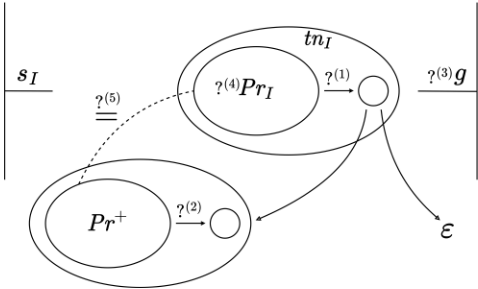
Figure 1 illustrates this problem class. In Figure 1, a question mark ? indicates that the corresponding element may or may not exist, with its index (∗) distinguishing it from other such elements. For example, in the configuration where "the elements marked ?(1) and ?(2) exist and element marked ?(3) does not exist": (i) There exists an ordering constraint in the initial task network requiring the compound task to follow all other primitive tasks (i.e., it is the last task). (ii) Similarly, within the method's task network, the compound task is ordered after all other primitive tasks. (iii) A goal does not exist, meaning the final state can be arbitrary as long as all tasks are executed. (iv) Primitive tasks may or may not be present in the initial task network. (v) The primitive tasks in the initial task network may form a sub-task network that may or may not be identical to the one in the method's task network.
We will analyze each of these structural restrictions in the following sections.
The class of planning problems characterized above elegantly aligns with the formal framework by Dekker and Behnke [2024]. The following definition provides a rigorous yet succinct formalization of the structural properties desired.
Definition 10 (r-Primitiveness). The class of recursive primitive task network planning problems, hereafter referred to as r-primitive problems, is the set H∩B∩L.
To ensure precise analysis, we will examine each restriction according to the following definitions. To enhance understanding, we will also explain each restriction by referring to the visualization above.
Definition 11 (r-Primitive Restrictions). Let P = (F,NC, NP ,M, δ; tnI, sI, g) be an r-primitive problem. Denote NC = {C } and M = {(C , ε), (C , tn+ )}. Then,
- P is goal-free iff g = ∅ (i.e, the element annotated by ?(3) in Figure 1 does not exist).
- P is execution-optional iff tnI ∈ TNC (i.e, the element annotated by ?(4) in Figure 1 does not exist).
- P is iteration-invariant iff there exists a primitive task network Pr ∈ TNP such that tnI and tn+ can each be obtained by augmenting Pr with C under some partial ordering (i.e., the element annotated by ?(5) in Figure 1 exists). Note that C can be inserted anywhere within the task network - even "in between" Pr - and its position may differ between the constructions of tnI and tn+ . This also means that transitivity may induce additional orderings, potentially making tnI and tn+ nonequivalent, even though both originate from Pr .
Our investigation proceeds through three analytical stages. We begin by establishing regularity conditions for the rprimitive problem class. Subsequently, we expand our analysis by relaxing the regularity constraint to tail-recursion. In the final stage, we complete the spectrum by withdrawing any constraints on the recursion type, thereby encompassing the entire class. We analyze the computational complexity as we progress through each stage, examining all subclasses that arise from the criteria in Definition 11.
First, we state the following proposition that trivially follows from the fact that in the respective case, the empty task network always forms a trivial solution.
Proposition 1. Deciding plan existence for goal-free and execution-optional r-primitive problems is in O(1).
3.1 On Regularity Conditions
This section examines regular r-primitive problems (elements marked ?(1) and ?(2) in Figure 1 both exist). As a subclass of regular HTN problems, this problem class retains PSPACE membership in terms of computational complexity. We prove that it is also PSPACE-hard.
Theorem 2. Deciding plan existence for regular executionoptional r-primitive problems is PSPACE-complete.
Proof. Membership inherits from the regular class. We prove hardness by reduction from classical planning.
Let P = (F,A, sI, g) be an instance of a classical planning problem, with F = {f1, . . . , fm} and A = {a1, . . . , an}. We construct a regular execution-optional r-primitive problem P∗ = (F ∗ ,NC,NP ,M, δ; tnI , s∗I , g∗ ), where F ∗ = F ∪ {token, flag}; NC = {C}; s∗I = sI ; g∗ = g; and
NP = {Initializer,Exclusion-Terminator,Restorer, Finalizer} ∪ {a∗1 , . . . , a∗n } ∪ {Enabler1, . . . , Enablern} ∪ {f1-Excluder, . . . , fm-Excluder}.M, δ, tnI are represented by Figure 1, with the following configurations: Elements marked ?(1) and ?(2) both exist; the element marked ?(4) does not exist; Pr + is shown in Figure 2.
Since C is ordered after the tasks in Pr + , the execution of tasks within Pr + cannot intertwine with any other potential occurrence of Pr + resulting from decomposition. We demonstrate that completing all tasks within Pr + at a state s is equivalent to selecting exactly one action from the set A and executing it at the state s.
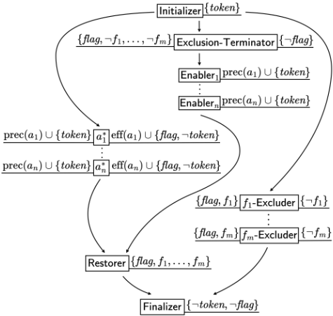
At s, the Initializer will be executed first, resulting in s ∪ {token}. Then, among the three branches, only the left one is executable because the others need the flag. Among actions in {a∗1 , . . . , a∗n }, exactly one of them, say a∗k , will be executed. This results in (s/eff - (ak)) ∪ eff + (ak) ∪ {flag}, consuming token to prevent others from executing. Denote this state as {fα1 , . . . , fαp }∪{flag}. At this state, only actions
in {fα1 -Excluder, . . . , fαp -Excluder} ⊆ {f1-Excluder, . . . , fm-Excluder} can be executed, resulting in the state {flag}. Now, only Exclusion-Terminator can be executed, removing flag to prevent any remaining fact excluders from executing. All actions in {Enabler1, . . . , Enablern} are then executable in arbitrary order. Note that for all i ∈ [1, k-1] ∪ [k+1,n], Enableri will always make a∗i executable right after. Therefore, there must exist an execution sequence to execute a∗1 , . . . , a∗k-1 , a∗k+1 , . . . , a∗n together with those enablers, so that Restorer can be executed afterwards. Its execution always results in the state {flag, f1, . . . , fm}, optionally including token as well. The remaining actions in {f1-Excluder, . . . , fm-Excluder}, namely {fi-Excluder ∣ i ∈ [1,m]/{α1, . . . ,αp}}, cannot be executed until Restorer has been executed. But once Restorer is executed, they can all be executed, resulting in the state {fi ∣ i ∈ [1,m]/([1,m]/{α1, . . . , αp})} ∪ {flag}, optionally including token as well. After removing token and flag by Finalizer, the state is exactly the same as (s/eff - (a)) ∪ eff + (a), i.e., the state resulting from executing ak at s.
Now we see that P has a solution iff P∗ has a solution. If P has a solution aβ1 , . . . , aβl , then P∗ also has a solution, where C is decomposed into Pr + l times and then into ε. The resulting primitive task network is equipped with a linearization such that the i-th execution of the actions in Pr + is equivalent to executing aβi for i ∈ [1, l]. Conversely, if P∗ has a solution tns consisting of l occurrences of Pr + , then P also has a solution of length l where each action is equivalent to the occurrence of Pr + in the corresponding ordering position.
The proof above illustrates a mechanism capable of selecting a specific range of actions and nullifying their effects. Previously, most methodologies for discarding unused actions failed to preserve the state following the discarding process, analogous to side effects in imperative programming. However, our novel approach demonstrates that it is feasible to discard unused actions without introducing side effects, ensuring that the state remains unchanged after the completion of the entire discarding mechanism. Furthermore, this proof enriches the standard toolkit available to researchers in HTN planning by addressing the frequent requirement for an "undo action" capability in various research contexts. The proof also possesses the potential for straightforward adaptation to meet these demands effectively. An example of such adaptation will be presented in the subsequent section.
The complexity result remains valid under the following conditions.
Corollary 1. Deciding plan existence for regular r-primitive problems is PSPACE-complete. This complexity result holds true even when the problems are further constrained to be iteration-invariant.
Proof. Without the iteration-invariant constraint, the result follows directly - Membership inherits from the regular class. Hardness is guaranteed by the fact that this problem class is a superclass of the class described in Theorem 2.
We then prove that the result holds under the iterationinvariant constraint. Membership inherits from the regular class. Hardness follows the same reduction as in the proof of Theorem 2, with the sole modification of adding to the input domain a null action that has no preconditions and no effects. This addresses the case of a zero-length plan (i.e., when the goal is already a subset of the initial state) by allowing the selection of the null action in the required iteration.
While computationally as hard as regular HTN problems, regular r-primitive problems cannot accommodate compiling goals away unless NP equals PSPACE. We prove this by presenting the following complexity result.
Theorem 3. Deciding plan existence for regular goal-free rprimitive problems is NP-complete. This complexity result holds true even when the problems are further constrained to be iteration-invariant.
Proof. It suffices to prove: (1) the NP membership of the problem class without the iteration-invariant constraint, and (2) the NP-hardness of the problem class with it.
(1) We prove this by reducing to the class of primitive task network planning problems. Let P be an arbitrary instance of a regular goal-free r-primitive problem. Assume that P is represented by Figure 1. Then, elements marked ?(1) and ?(2) both exist, but the element marked ?(3) does not. If PrI possesses an executable linearization, P has a solution. If PrI does not possess an executable linearization, P must be unsolvable because the order restriction prevents it from intertwining with other occurrences of itself. Hence, planning for P is equivalent to planning for PrI .
(2) We prove this by reduction from the class of primitive task network planning problems. Given any primitive task network Pr, we can construct a regular iteration-invariant goal-free r-primitive problem P to simulate planning for one or more sequentially ordered occurrences of Pr. The only modification we need is to add a fact, a token, and a limiting action, with the token in its precondition and delete set. This restricts Pr to iterate at most once. Then, P has a solution iff Pr possesses an executable linearization.
Most HTN problem formalizations exclude explicit goal representations, assuming that goals can be readily compiled into other constructs. However, we demonstrate that goal compilation is not universally achievable. Therefore, the inclusion or exclusion of explicit goal representations should be contextually evaluated, accounting for the specific constraints and characteristics of each problem class.
3.2 On Tail-Recursion Conditions
We proceed by examining the tail-recursive r-primitive problems (i.e., the element marked ?(2) in Figure 1 exists). Note that the class of regular execution-optional r-primitive problems is identical to that of tail-recursive execution-optional rprimitive problems. Therefore, this class will not be revisited in this section. Our analysis begins with goal-free problems and then extends to those that do not respect this constraint.
Theorem 4. Deciding plan existence for tail-recursive goalfree r-primitive problems is PSPACE-complete. This complexity result holds true even when the problems are further constrained to be iteration-invariant.
Proof. It suffices to prove: (1) the PSPACE membership of the problem class without the iteration-invariant constraint, and (2) the PSPACE-hardness of the problem class with it.
(1) Let P be a tail-recursive goal-free r-primitive problem. Assume Figure 1 represents the structure of P. Then, the element marked ?(2) exists, but the element marked ?(3) does not. Consider applying progression search to P. The key observation is that, since C is ordered after all actions in Pr + within the method, it cannot be replaced by a new occurrence of Pr + before all actions in the existing Pr + have been removed from the search fringe. Therefore, the search fringe can contain at most all tasks from PrI , all tasks from Pr + , and C, which are ∣PrI ∣ + ∣Pr∣ + 1 tasks. This means that, during its execution, the progression search only uses space bounded by a polynomial in the input size. Hence, by Savitch's reachability algorithm, the progression search is guaranteed to terminate on P. Thus, PSPACE membership holds for this class.
(2) We prove this by reduction from the class of regular iteration-invariant r-primitive problems, which has been proven to be PSPACE-complete in Corollary 1. Let P = (F,NC,NP ,M, δ; tnI, sI, g) be an arbitrary instance of a regular iteration-invariant r-primitive problem. Let g = {g1, . . . , gm}. Since P is iteration-invariant, there must exist a task network Input-Pr satisfying the conditions specified in the definition of iteration-invariant. We construct a tail-recursive goal-free r-primitive problem P∗ = (F ∗ ,N ∗C ,N ∗ P ,M ∗ , δ∗ ; tn∗I , s∗I , g∗ ) accordingly, where F ∗ = F ∪ g; N ∗C = {C}; s∗I = sI; g∗ = ∅; and NP = {Restorer,Goal-Guarantor} ∪ {g1-Excluder, . . . , gm-Excluder}. M, δ, tnI are represented by Figure 1, with the following configurations: The elements marked ?(2) , ?(4) , ?(5) all exist; the element marked ?(3) does not exist; PrI (as well as Pr + ) is depicted in Figure 3.
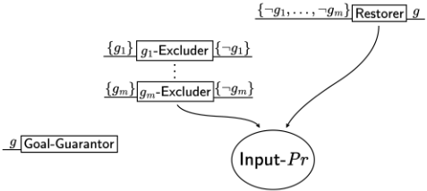
In tnI, C is ordered after Input-Pr and before GoalGuarantor. By transitivity, Goal-Guarantor is ordered as the last task in tnI. Clearly, the construction of P∗ ensures that Goal-Guarantor remains the last task in any task network resulting from applying any sequence of decomposition methods. By executing Goal-Guarantor eventually, it is guaranteed that g is a subset of the final state. However, g need not be a subset of the intermediate states resulting from each execution of Input-Pr. Moreover, after executing an occurrence of Input-Pr, the state remains unchanged until any potential subsequent occurrences of Input-Pr are executed. We provide the justification below.
When executing PrI or Pr + in state s, a subset of actions {gα1 -Excluder, . . . , gαp -Excluder} ⊆ {g1-Excluder, . . . , gm-Excluder}, where {gα1 , . . . , gαp } ⊆ s, will be executed to reach the state s∗ ∶= s/g. Then, Restorer becomes executable and, when executed, results in state s∗ ∪ g. This allows Goal-Guarantor to be executed, unless the current task network is the initial one where it is already ordered as the last task. Finally, the remaining goal excluders, namely actions in {gi-Excluder ∣ i ∈ [1,m]/{α1, . . . ,αp}}, can be executed, transforming state s∗ ∪ g into
Therefore, when proceeding to execute Input-Pr, the state remains s, the same as before executing PrI or Pr + .
The above justifies the validity of goal compilation, and thus P has a solution iff P∗ does.
This proof demonstrates another application of the statepreserving action nullification mechanism. While it represents a lighter implementation - conditionally discarding only the action encoding the goal - it employs the same principles as in the previous section thus reinforcing the mechanism's effectiveness and broad applicability.
Unlike regular r-primitive problems, the current class does not become computationally easier in the absence of goals, as demonstrated by the theorem below.
Corollary 2. Deciding plan existence for tail-recursive rprimitive problems is PSPACE-complete. This complexity result holds true even when the problems are further constrained to be iteration-invariant.
Proof. It suffices to compile away the goals for the problem class without the iteration-invariant constraint. This can be achieved by simply adding an additional action with the goal as its precondition and ordering it as the last task in the initial task network. After this modification, the problem still satisfies the requirement of being tail-recursive.
This corollary also indicates that relaxing the ordering restrictions of the compound task within the initial task network for the regular r-primitive problem class does not yield a harder class, but instead preserves the same complexity.
3.3 On Arbitrary Recursion Types
We complete our investigation by analyzing the general class of r-primitive problems. A direct application of Theorem 1 reveals that deciding plan existence for goal-free r-primitive problems is ACKERMANN-complete. We extend this result to encompass additional subclasses, beginning with a proof for a more restricted subclass.
Theorem 5. Let U denote the intersection of the class of r-primitive problems and I ∩ F. Then, deciding plan existence for goal-free and iteration-invariant problems within U is ACKERMANN-complete.
Proof. Membership follows from a direct application of Theorem 1. We prove ACKERMANN-hardness by reduction from the class of goal-free problems in I ∩ F ∩ H ∩ B ∩ L, which is known to be ACKERMANN-complete by Theorem 1. Let P = (F,NC,NP ,M, δ; tnI, sI, g) be an arbitrary instance of this class. In this case, g = ∅. Let a1, . . . , am denote the primitive tasks appearing in the initial task network. We refer to them collectively as PrI. Similarly, let b1, . . . , bn be the primitive tasks in the nonempty task network within the method, collectively referred to as Pr+ . We construct a goal-free iteration-invariant r-primitive problem P∗ = (F ∗ ,N ∗C ,N ∗ P ,M ∗ , δ∗ ; tn∗I , s∗I , g∗ ) accordingly, where F ∗ = F ∪ {flag, s1, s2, s3} ∪ {token1, . . . , tokenm}; N ∗C = {C}; s∗I = sI ∪ {token1, . . . , tokenm}; g∗ = ∅; and
M, δ, tnI are represented by Figure 1, with the following configurations: The elements marked ?(4) and ?(5) both exist; the elements marked ?(1) , ?(2) , ?(3) do not exist; PrI (as well as Pr + ) is depicted in Figure 4.
Actions within Input-PrI and Input-Pr + inherit the original partial ordering. When planning for P∗ , the states of P∗ can be classified into 5 stages: (1) action stage - states excluding s1, s2, s3; (2) Pr + -trashing stage - states including s1 but not s2, s3; (3) PrI -trashing stage - states including s2 but not s1, s3; (4) supplementary stage - states including s3 but not s1, s2; (5) finalizing stage - states including s1, s3 but not s2. In the action stage, Input-PrI can be executed exactly once regardless of the number of occurrences. Input-Pr + can be executed either an unlimited number of times or not at all. Note that it is not possible for only part of Input-Pr + to be executed, because every action in it adds flag to the state, which prevents entry into the Pr + -trashing stage used to discard actions that are not executed. Depending on whether Input-Pr + has been executed at least once, two scenarios arise:
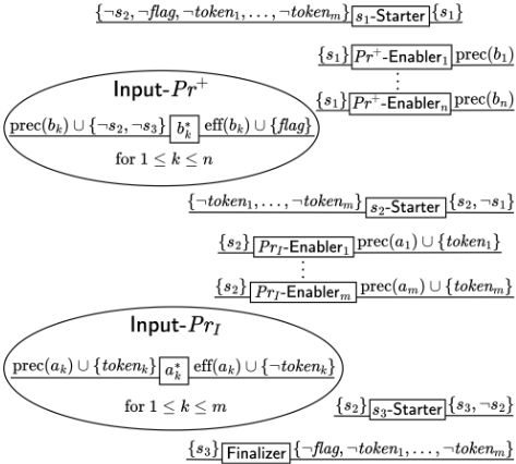
In the first scenario, where Input-Pr + is not executed at all, the process enters the Pr + -trashing stage to discard all occurrences of Input-Pr + . It then proceeds to the PrI -trashing stage to discard any remaining occurrences of Input-PrI (in case there exists at least one occurrence of Pr + , i.e., additional copies of Figure 4). Finally, it enters the supplementary stage and executes Finalizer. This scenario corresponds to the case in which P has a solution that contains only Input -PrI .
In the second scenario, where Input-Pr + is executed at least once, the process enters the PrI -trashing stage to discard any remaining occurrences of Input-PrI . Then, it enters the supplementary stage and executes Finalizer, which enables entry into the finalizing stage to assist in discarding actions related to the Pr + -trashing stage. This scenario corresponds to the case where P has a solution that includes Input-PrI and one or more occurrences of Input -Pr + .
Therefore, P∗ precisely simulates the mechanism of P, which implies that P∗ has a solution iff P has a solution.
The above theorem reveals the complexity of problems further constrained by the condition that each occurrence of the compound task is isolated from other (primitive) tasks within the same task network. This result, specific to the compoundisolated subclass, illustrates the minimum complexity of the broader class in which that constraint is removed. Consequently, we establish the following corollary.
Corollary 3. Deciding plan existence for goal-free iterationinvariant r-primitive problems is ACKERMANN-complete.
Proof. Membership follows from direct application of Theorem 1. Hardness follows from the fact that the class described in Theorem 5 is a subclass of this class.
The r-primitive problem class possesses sufficient expressive power to accommodate goal compilation, ensuring that the complexity class remains unchanged when working with goals, as demonstrated below.
Corollary 4. Deciding plan existence for r-primitive problems is ACKERMANN-complete. This complexity result holds true even when the problems are further constrained to be execution-optional or iteration-invariant.
Proof. Membership follows from the canonical compilation of goals. Given an arbitrary r-primitive problem, one can compile away the goal by constructing a goal-simulating action - an action whose precondition is exactly the goal - and placing it as the last task in the initial task network. Note that this compilation may yield a problem that is neither execution-optional nor iteration-invariant, but the resulting problem still belongs to the class H, which is ACKERMANN-complete.
For the class of r-primitive problems and the class of iteration-invariant r-primitive problems, their hardness follows from the hardness of their corresponding goal-free versions (i.e., each class with the additional goal-free constraint). To prove the hardness of the class of execution-optional rprimitive problems, consider the class described in Theorem 5. Removing the goal-free constraint from this class preserves the ACKERMANN-hardness. Given an arbitrary problem (possibly with a non-empty goal) in this class, we can reduce it to an execution-optional r-primitive problem by adding a new fact to the goal and constructing an action whose effect is to add this fact. Then, the primitive tasks in the initial task network can be safely removed, as long as the aforementioned action is included as an isolated task (i.e., unordered with respect to the other tasks) within the method's task network. This ensures that the non-trivial decomposition must be applied at least once.
4 Conclusion
We investigated the computational complexity of a class we term the r-primitive problem class. To this end, we systematically analyzed a range of factors that may contribute to the problem's complexity, thereby uncovering connections to - and offering new insights into - existing problem classes. In addition, we introduce a novel proof technique that may enrich the toolkit for analyzing HTN problems. This technique enables the application of a set of actions, of which only one is semantically applied (i.e., only one affects the state), while the effects of all others are reversed. We refer to this method as selective action nullification with state preservation and suggest that it may have applications beyond the specific proofs in which it has already been employed.
Acknowledgments
Pascal Bercher is the recipient of an Australian Research Council (ARC) Discovery Early Career Researcher Award (DECRA), project number DE240101245, funded by the Australian Government.
@inproceedings{ijcai2025p967,
  title     = {Computational Complexity of Planning for Recursive Primitive Task Networks: Selective Action Nullification with State Preservation},
  author    = {Zhang, Yifan and Bercher, Pascal},
  booktitle = {Proceedings of the Thirty-Fourth International Joint Conference on
               Artificial Intelligence, {IJCAI-25}},
  publisher = {International Joint Conferences on Artificial Intelligence Organization},
  editor    = {James Kwok},
  pages     = {8696--8704},
  year      = {2025},
  month     = {8},
  note      = {Main Track},
  doi       = {10.24963/ijcai.2025/967},
  url       = {https://doi.org/10.24963/ijcai.2025/967},
}
TY - CPAPER TI - Computational Complexity of Planning for Recursive Primitive Task Networks: Selective Action Nullification with State Preservation AU - Zhang, Yifan AU - Bercher, Pascal T2 - Proceedings of the Thirty-Fourth International Joint Conference on Artificial Intelligence, IJCAI-25 PB - International Joint Conferences on Artificial Intelligence Organization PY - 2025 SP - 8696 EP - 8704 DO - 10.24963/ijcai.2025/967 UR - https://doi.org/10.24963/ijcai.2025/967 ER -Copied
Machine-readable versions of this paper, for tools and AI agents:





