
Speeding Up Hyper-Heuristics With Markov-Chain Operator Selection and the Only-Worsening Acceptance Operator
Proceedings of the Thirty-Fourth International Joint Conference on Artificial Intelligence. Main Track. Pages 8850-8857.
https://doi.org/10.24963/ijcai.2025/984
Keywords
- Search: S: Evolutionary computation
- Search: S: Heuristic search
Abstract
The move-acceptance hyper-heuristic was recently shown to be able to leave local optima with astonishing efficiency (Lissovoi et al., Artificial Intelligence (2023)). In this work, we propose two modifications to this algorithm that demonstrate impressive performances on a large class of benchmarks including the classic CLIFF_d and JUMP_m function classes. (i) Instead of randomly choosing between the only-improving and any-move acceptance operator, we take this choice via a simple two-state Markov chain. This modification alone reduces the runtime on JUMP_m functions with gap parameter m from ?(n²ᵐ⁻¹) to O(nᵐ⁺¹). (ii) We then replace the all-moves acceptance operators with the operator that only accepts worsenings. Such a, counter-intuitive, operator has not been used before in the literature. However, our proofs show that our only-worsening operator can greatly help in leaving local optima, reducing, e.g., the runtime on Jump functions to O(n³ log n) independent of the gap size. In general, we prove a remarkably good runtime of O(nᵏ⁺¹ log n) for our Markov move-acceptance hyper-heuristic on all members of a new benchmark class SEQOPT_k, which contains a large number of functions having k successive local optima, and which contains the commonly studied JUMP_m and CLIFF_d functions for k=2.
- [Auger and Doerr, 2011] Anne Auger and Benjamin Doerr, editors. Theory of Randomized Search Heuristics. World Scientific Publishing, 2011.
- [Burke et al., 2013] Edmund K. Burke, Michel Gendreau, Matthew R. Hyde, Graham Kendall, Gabriela Ochoa, En- der Özcan, and Rong Qu. Hyper-heuristics: a survey of the state of the art. Journal of the Operational Research Society, 64:1695-1724, 2013.
- [Cowling et al., 2000] Peter I. Cowling, Graham Kendall, and Eric Soubeiga. A hyperheuristic approach to schedul- ing a sales summit. In Practice and Theory of Automated Timetabling, PATAT 2000, pages 176-190. Springer, 2000.
- [Doerr and Künnemann, 2015] Benjamin Doerr and Marvin Künnemann. Optimizing linear functions with the (1 + λ) evolutionary algorithm-different asymptotic runtimes for different instances. Theoretical Computer Science, 561:3- 23, 2015.
- [Doerr and Neumann, 2020] Benjamin Doerr and Frank Neumann, editors. Theory of Evolutionary Computation- Recent Developments in Discrete Optimization. Springer, 2020. Also available at http://www.lix.polytechnique.fr/ Labo/Benjamin.Doerr/doerr neumann book.html. Link
- [Doerr et al., 2018] Benjamin Doerr, Andrei Lissovoi, Pietro S. Oliveto, and John Alasdair Warwicker. On the runtime analysis of selection hyper-heuristics with adaptive learning periods. In Genetic and Evolution- ary Computation Conference, GECCO 2018, pages 1015-1022. ACM, 2018.
- [Doerr et al., 2023a] Benjamin Doerr, Arthur Dremaux, Jo- hannes F. Lutzeyer, and Aurélien Stumpf. How the move acceptance hyper-heuristic copes with local optima: dras- tic differences between jumps and cliffs. In Genetic and Evolutionary Computation Conference, GECCO 2023, pages 990-999. ACM, 2023.
- [Doerr et al., 2023b] Benjamin Doerr, Taha El Ghazi El Houssaini, Amirhossein Rajabi, and Carsten Witt. How well does the Metropolis algorithm cope with local op- tima? In Genetic and Evolutionary Computation Con- ference, GECCO 2023, pages 1000-1008. ACM, 2023.
- [Drake et al., 2020] John Drake, Ahmed Kheiri, Ender Özcan, and Edmund Burke. Recent advances in selec- tion hyper-heuristics. European Journal of Operational Research, 285:405-428, 09 2020.
- [Droste et al., 2002] Stefan Droste, Thomas Jansen, and Ingo Wegener. On the analysis of the (1+1) evolution- ary algorithm. Theoretical Computer Science, 276:51-81, 2002.
- [Jansen, 2013] Thomas Jansen. Analyzing Evolutionary Al- gorithms -The Computer Science Perspective. Springer, 2013.
- [Kötzing and Krejca, 2019] Timo Kötzing and Martin S. Krejca. First-hitting times under drift. Theoretical Com- puter Science, 796:51-69, 2019.
- [Lehre and Özcan, 2013] Per Kristian Lehre and Ender Özcan. A runtime analysis of simple hyper-heuristics: to mix or not to mix operators. In Foundations of Genetic Algorithms, FOGA 2013, pages 97-104. ACM, 2013.
- [Lissovoi et al., 2019] Andrei Lissovoi, Pietro S. Oliveto, and John Alasdair Warwicker. On the time complexity of algorithm selection hyper-heuristics for multimodal opti- misation. In Conference on Artificial Intelligence, AAAI 2019, pages 2322-2329. AAAI Press, 2019.
- [Lissovoi et al., 2020] Andrei Lissovoi, Pietro S. Oliveto, and John Alasdair Warwicker. How the duration of the learning period affects the performance of random gradi- ent selection hyper-heuristics. In Conference on Artificial Intelligence, AAAI 2020, pages 2376-2383. AAAI Press, 2020.
- [Lissovoi et al., 2023] Andrei Lissovoi, Pietro S. Oliveto, and John Alasdair Warwicker. When move acceptance se- lection hyper-heuristics outperform Metropolis and elitist evolutionary algorithms and when not. Artificial Intelli- gence, 314:103804, 2023.
- [Neumann and Witt, 2010] Frank Neumann and Carsten Witt. Bioinspired Computation in Combinatorial Opti- mization -Algorithms and Their Computational Complex- ity. Springer, 2010.
- [Wald, 1944] Abraham Wald. On cumulative sums of ran- dom variables. Annals of Mathematical Statistics, 15:283- 296, 1944.
- [Zhou et al., 2019] Zhi-Hua Zhou, Yang Yu, and Chao Qian. Evolutionary Learning: Advances in Theories and Algo- rithms. Springer, 2019.
References were extracted automatically from the PDF and may contain errors.
Full text extracted automatically from the PDF; figures, tables and equations may differ. The PDF is the version of record.
1 Introduction
Selection hyper-heuristics are black-box optimization heuristics that function by combining different low-level heuristics. They were first used to solve difficult scheduling problems [Cowling et al., 2000], but then quickly found numerous other applications [Burke et al., 2013; Drake et al., 2020].
The mathematical runtime analysis of hyper-heuristics has started around ten years ago [Lehre and ¨Ozcan, 2013], predominantly discussing the impact of selecting different variation operators [Doerr et al., 2018; Lissovoi et al., 2020]. More recently, hyper-heuristics having the choice between different acceptance operators were studied (although a first result can already be found in [Lehre and ¨Ozcan, 2013]). In particular, [Lissovoi et al., 2019; Lissovoi et al., 2023] have shown that switching between an elitist selection (the onlyimproving operator OI) and accepting any new solution (the all-moves operator AM) can give excellent results. Specifically, they show that the move-acceptance hyper-heuristic (MAHH) can optimize the CLIFFd benchmark defined on bitstrings of length n in time O(n3 ), whereas comparably simple elitist evolutionary algorithm need time Ω(nd ); here d is a difficulty parameter of the benchmark that can range from 2 to n. A similar lower bound was shown for the Metropolis algorithm [Doerr et al., 2023b].
∗An extended version of this manuscript, including appendices, can be accessed on the arXiv repository.
However, such performance gains seem to heavily depend on the particular problem to be optimized. For the jump benchmark with difficulty parameter m, simple evolutionary algorithms find the optimum in expected time O(nm) [Droste et al., 2002], but the MAHH needs Ω(n2m-1 ) [Doerr et al., 2023a] (for constant m).
In this work, we propose two new ideas that help hyperheuristics to leave local optima, and greatly improve their performance. We also observe that the proposed modifications resolve the difficulties detected in [Doerr et al., 2023a]. (i) From studying the proofs in [Doerr et al., 2023a], we observe that the use of the randommixing strategy, that is, using the all-moves operator in each iteration independently with some probability p, is problematic. The probability p has to be small to allow for a sufficiently strong drift towards the optimum, but leaving a local optimum with radius m requires m- 1 successive uses of the AM operator, which contributes a factor of pm-1 to the probability of successfully leaving the local optimum. To mitigate the influence of the required small rate of AM operator uses, we design a simple two-state Markov chain governing the selection of the operators. In other words, for each of the two acceptance operators, we have a switching probability. In each iteration, we use this value to decide whether we should switch to the other operator or continue with the current operator. By taking a value such as 1/2 for the probability of switching away from the AM operator, longer stretches of using this operator become more likely, which eases the leaving of local optima with larger basins of attraction. We call the resulting algorithm Markov move-acceptance hyper-heuristic (MMAHH). As an example of the usefulness of this approach, we show that the MMAHH choosing the two operators OI and AM (with the long-term rates of the operators as in previous works) optimizes JUMP functions in time O(nm+1 ), a considerable speed-up from Ω(n2m-1 ). We note that in general this way of choosing between operators has been used before, but to the best of our knowledge no mathematical runtime result has been shown, and it has not been used in conjunction with acceptance operators until now.
We then propose the only-worsening (OW) acceptance operator. It accepts the new solution only if it is strictly worse than the parent. While this operator contradicts the idea of incremental optimization, in our context it is less counterintuitive than what appears at first. We recall that the main working principle of the AM operator exploited in previous works is that it allows the algorithm to leave local optima. For this aim, searching for inferior solutions is, in fact, a logical approach. This intuitive consideration is supported by our mathematical runtime analysis, which in particular shows that the MMAHH with the two acceptance operators OI and OW optimizes any JUMP and CLIFF function in expected time O(n3 log n). We extend this result to a new benchmark called SEQOPTk, which consists of a broad class of pseudoBoolean functions having k local optima that in particular includes the classic ONEMAX, JUMP, CLIFF, and TRAP benchmarks. We show that our MMAHH optimizes any function in SEQOPTk in expected time O(nk+1 log n).
With this work, we introduce two new ideas for the design of effective move-acceptance hyper-heuristics. We believe that in particular, the only-worsening operator to leave local optima, could give rise to further theoretical study and possibly the design of new benchmarks designed to test its limits. We furthermore hope that future consideration of our SEQOPTk benchmark enables a joint observation of the effectiveness of hyper-heuristics that subsumes results on the different commonly studied JUMP and CLIFF benchmarks.
2 Preliminaries
In this section, we briefly recall the classic benchmark problems relevant for this work, define our new benchmark SEQOPTk, define our Markov move-acceptance hyperheuristic, the only-worsening acceptance operator, and provide the tools to analyze our hyper-heuristics.
2.1 Benchmarks
As standard in the theory of randomized search heuristics [Neumann and Witt, 2010; Auger and Doerr, 2011; Jansen, 2013; Zhou et al., 2019; Doerr and Neumann, 2020], we regard pseudo-Boolean optimization problems, that is, we aim at maximizing functions f that map bit-strings x ∈ {0, 1}n with a fixed positive length n ∈ N>0 = {1, 2, 3, . . .} to a numerical value f(x) ∈ R. When using asymptotic notation, this shall always be for n→∞.
Well-known examples of such functions in the theory literature include the following ONEMAX, TRAP, CLIFFd and JUMPm benchmarks.
For a bit-string x = (x1, . . . , xn) ∈ {0, 1}n , let ∥x∥1 = x1 + x2 + · · · + xn denote the number of ones in x. The following functions are standard benchmarks in the theory of randomized search heuristics.
Here d ∈ [1..n-1] and m ∈ [1..n] are difficulty parameters of the CLIFF and JUMP benchmark. The completely deceptive function JUMPn is also called TRAP. All these functions have x∗ = (1, . . . , 1) as unique global optimum (maximum), and all are functions of unitation, that is, the objective value of a solution depends only on the number of ones. This motivates the definition of the k-th layer as
for k ∈ [0..n], where we used H(·, ·) to denote the Hamming distance of two bit-strings. Note that Lk is the set of all bitstrings at distance k from the global maximum x∗ , that is, the numbering starts at the global optimum.
All benchmarks above also have the property that they are composed of intervals of layers in which the function is only increasing or only decreasing; for JUMPm and CLIFFd these intervals have lengths 2, m-1, and n-m+1. In the following two definitions, we extend this property to arbitrary interval numbers and lengths and obtain the very general benchmark SEQOPTk, having k successive local minima and maxima.
Definition 1 (Monotonicity across layers). Let h ∈ [0..n - 1] and f : {0, 1}n → R. We say that f is increasing (resp. decreasing) between layers Lh+1 and Lh if for any x ∈ Lh and y ∈ Lh+1 we have
We denote this by Lh f≻ Lh+1 (resp. Lh f≺ Lh+1).
Definition 2 (The SEQOPT benchmark). Let n ≥ 2, k ∈ [0..n - 2] and d0 = n > d1 > d2 > · · · > dk > dk+1 = 0 be integers. We define SEQOPTk(d1, . . . , dk) to be the set of all functions f : {0, 1}n → R such that
(i) x∗ = (1, . . . , 1) is the unique global maximum of f,
(ii) for any ℓ ∈ [0..k], if k - ℓ is even then
and if k - ℓ is odd, f satisfies
The union of these classes of functions, for fixed k, will be denoted by
Note that we have ONEMAX ∈ SEQOPT0, TRAP ∈ SEQOPT1(1), CLIFFd ∈ SEQOPT2(d, d - 1) and, for m < n, JUMPm ∈ SEQOPT2(m, 1).
2.2 The MarkovMove-Acceptance Hyper-Heuristic
We now introduce a novel algorithm called the Markov MoveAcceptance Hyper-Heuristic algorithm (MMAHH). We recall that the Move-Acceptance Hyper-Heuristic algorithm (MAHH) first proposed in [Lehre and ¨Ozcan, 2013] and then intensively studied in [Lissovoi et al., 2023] is a simple randomized local search heuristic which randomly mixes between the OI and AM operators, that is, in each iteration independently is chooses between the AM operator (with some, usually small, probability p) and the OI operator (with probability 1 - p).
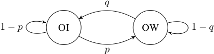
From studying the proof of the unsatisfactory Ω(n2m-1 ) runtime bound for this algorithm on the JUMPm benchmark, we learn that the main reason for this negative performance is the low probability of having m- 1 consecutive uses of the AM operator, which stems from the independent choice of the operators. To allow for longer phases of using the same operator, our MMAHH leverages a simple 2-state Markov chain to govern the selection of the acceptance operators. In other words, if the current operator is OI, this operator is kept for the next iteration with probability 1 - p, but changed to AM with probability p. The switching probability from AM to OI is denoted by q. See Algorithm 1 for the pseudocode of the MMAHH, where the MARKOV operator refers to sampling the Markov chain illustrated in Figure 1.
We also introduce a new acceptance operator, onlyworsening (OW), to substitute the ALLMOVES (AM) operator. This new operator works in the same fashion as the wellknown ONLYIMPROVING (OI) acceptance operator except that OW only accepts worsening moves, i.e., moves decreasing the function value. The idea of this, counter-intuitive, operator is to speed-up leaving local optima. When studying the previous runtime analyses for the MAHH, we see that they profit from the AM operator in that it allows the algorithm to leave local optima. If this is the target, then the OW operator should be even better suited, and this is what we will observe in this work.
2.3 Notation for the Analysis of the MMAHH
Throughout this work, we denote by xt, yt and st, respectively, the current solution at time t, its Hamming distance to x∗ (i.e., yt = H(xt, x∗ )), and the move-acceptance operator used at time t. We initialize with a random solution x0 ∼ U({0, 1}n ) and s0 = OI. We always denote by f : {0, 1}n → R the function to be maximized. Moreover, the transition probabilities from OI to OW and OW to OI will be denoted respectively by p and q with 0 < p, q < 1.
| Symbol | Meaning |
|---|---|
| T s p, Zk f x∗ | The first hitting time of x∗ starting time of the k-th phase probabilities of the Markov |
| T (k) | The |
| q | Transition chain |
| The length of the k-th phase | |
| A function with a unique global maximum | |
| The global maximum of f, x∗ = {1}n | |
| xt | The bit-string during the t-th iteration |
| yt | The Hamming distance to x∗ at time t |
| st | The move-acceptance operator at time t |
| x0 | The initial bit-string, x0 ∼ U({0, 1}n ) |
| s0 | The initial move-acceptance operator, s0 = OI |

We call T := inf{t ≥ 0 | xt = x∗ } the runtime, that is, the first time we reach the global maximum. Let T (k) s denotes the k-th switching time between the operators. Hence T (0) s = 0 and for any k ≥ 0, we have T (k+1) s = inf{t ≥ T (k) s | st ̸= sT (k) s }. We also define Zk = T (k+1) s -T (k) s to be the length of the k-th phase, where a phase is a (maximum) time interval in which the same operator is used.
This notation is summarized in Table 1 and illustrated in Figure 2.
Algorithm 1: The Markov move-acceptance hyperheuristic with the acceptance operators OI and OW.
1 Initialization: 2 t ← 0 3 x0 ∼ U({0, 1}n ), a uniformly sampled bit-string 4 s0 ← OI 5 while true do 6 x′ ← RAMDOMONEBITFLIP(xt) 7 if st = OW and f(x′ ) < f(xt) then 8 xt+1 ← x′ 9 else if st = OI and f(xt) < f(x′ ) then 10 xt+1 ← x′ 11 st+1 ← MARKOV(st) 12 t ← t + 12.4 Tools for the Analysis of the MMAHH
We now develop the tools we need to analyze the MMAHH. Unfortunately, the generality of the Markov chain of our setup disallows the use of the methods previously employed in the analysis of the MAHH, which were mostly drift arguments based on the fitness of the current solution. Nonetheless, with some mathematical effort, we manage to obtain very precise estimates of the quantities of interest.
Probability of improvement in one phase. We start by computing the probabilities that a single phase of OI usages leads to a certain fitness improvement. From the way we constructed the Markov chain, the length Zk of each phase is independent from the solution xT (k) s it starts with (and hence its fitness yT (k) s ), and follows a geometric law.
For 0 ≤ h, k ≤ n, let phk = Pr[yT (1) s ≤ h | y0 = k, s0 = OI] denote the probability to reach Lh in one OI phase when starting in state OI in Lk, assuming that we optimize the ONEMAX benchmark. The following computation of these probabilities is a cornerstone of our analysis.
Lemma 3. For all 0 < p < 1 and 0 ≤ h, k ≤ n, we have
The next key lemma shows that p = Θ( 1 n log(n) ), that is, a quasi-linear length of the OI phase, suffices to have a constant probability p0n to optimize ONEMAX in one OI phase even when starting in the all-zero string.
From a simple domination argument, exploiting that our hyper-heuristics have to visit all intermediate levels, we immediately obtain the following minimality statement.
Lemma 5 (Minimality of p0n ). For all 0 ≤ h, k ≤ n, we have phk ≥ p0n .
As OI and OW operators work in a symmetric fashion, similar results hold on OW and decreasing moves. More specifically, given 0 ≤ h, k ≤ n, we have
In particular, when q = Θ( 1 n log(n) ), the probability to climb down ONEMAX entirely in one phase of OW is Ω(1).
We can further extend Lemma 3 to the SEQOPT benchmark. Note that for any k and f ∈ SEQOPTk, for each ℓ the transition probability between layer Lℓ and Lℓ-1 (resp. Lℓ and Lℓ+1, when defined), are the same as for ONEMAX, namely, ℓn (resp. n-ℓ n ). Thus, the computations done in Lemma 3 still hold for f in regions where f is monotonic across the layers, as defined in Definition 1.
We further note that, for ONEMAX again, the average number of pairs of phases of OI followed by OW needed to reach the optimum is bounded from above by 1 p0n , since in the worst scenario, every phase of OW bring us back to the all-zero string. Extending this insight again to SEQOPT, we see that in the quasi-linear regime, reaching a neighboring local optimum starting from a local optimum of any SEQOPT function only takes O(1) pairs of phases. This particular fact will be referred as to the one-phase approximation, stated more formally in the next lemma.
Lemma 6 (One-phase approximation). Let p = Θ( 1 n log(n) ) and q = Θ( 1 n log(n) ). Let f ∈ SEQOPTk(d1, . . . , dk), ℓ ∈ [0..k] and x0 ∈ Ldℓ . Then the MMAHH algorithm reaches some x ∈ Ldℓ-1 ∪ Ldℓ+1 in O(1) phases on average.
3 MMAHHWith OI+AMon Jump
The core objective of this section is to prove that the sole use of the Markov chain improves significantly the performance of the MAHH on JUMPm, reducing its average runtime from Ω( n2m-1 (2m-1)! ) to O(nm+1 ) as outlined in the next theorem.
To clearly point out the contribution of the Markov chain, we consider the MMAHH on JUMPm where 1 < m < n2 using the OI and AM operators, with probability p and q to choose them respectively (we just replace OW in Figure 1 by AM).
Theorem 7 (Runtime analysis of the MMAHH on JUMPm with OI-AM). The time T taken by the MMAHH on JUMPm with 1 < m < n2 to reach x∗ , using OI and AM, satisfies
where Nn,m,q = n + nm (m-1)!(1-q)m-2 , n ≥ 3 and p, q are such that m 2(n-2m) (q + 4n ) ≥ p.
Notably, it suffices to have m 2n q ≥ p from where we have:
- (i) When p = m cn q for some c ≥ 2 and q = 12 then
(ii) When p = m cn q and q = 1 dm where c ≥ 2 and d ≥ 1 then
The proof of the theorem relies mainly on drift theorems. Hence we start by studying the drift in the following lemmas. Throughout this part, the drift over a phase of AM (resp. OI) starting in i ∈ [0..n] (denoting the number of zero bits) will be ∆AM i (resp. ∆OI i ) and defined as
Lemmas 8, 9 and 10 give the drift over a phase of AM, a phase of OI and a pair AM+OI of phases.
Lemma 8 (Drift over a phase of AM). Let i ∈ [0..n] and an integer k ≥ 0, the drift over a phase of AM on ONEMAX is
Lemma 9 (Drift over a phase of OI). Let i ∈ [0..n] and an integer k ≥ 0, the drift over a phase of OI on ONEMAX is
Lemma 10 (Drift over a pair AM+OI of phases). For any i ∈ [0..n] and k ≥ 0 an integer, the drift over a phase of AM followed by a phase of OI on ONEMAX is
i.e., we can split the drift across two phases and plug the average position after a phase of AM directly in the drift of a phase of OI.
Now, the following lemma provides an upper bound on the average number of phases of AM needed to reach the global maximum at x∗ = {1}n from a local maximum in layer Lm.
Lemma 11. The probability to reach the global maximum x∗ during a single phase of AM starting from a local maximum in layer Lm is
Let
the set of (local and global) maxima of JUMPm and we consider the potential
In the next two lemmas, we work out lower bounds on the drift of the bit-string sequence, distinguishing two cases based on the landscape of the JUMPm function. In Lemma 12, we lower bound the drift in the gap region, i.e., at positions x ∈ {0, 1}n such that n-m < ∥x∥1 < n, directly on the sequence (xt)t≥0 using the potential d defined earlier. This result will provide an upper bound on the average time needed to climb towards x∗ from a point x0 in the gap region. On the other hand, Lemma 13 deals with the drift in the region with the ONEMAX-like slope, i.e., bit-strings x ∈ {0, 1}n for which 0 ≤ ∥x∥1 < n -m. This time, we work at the scale of a pair of phases AM+OI since locally, depending on the current operator OI or AM, the drift might have opposite signs, notably in the region [ n2 ..(n - m)]. To this aim, we will use Lemma 10 along with the additive drift theorem with overshooting [K¨otzing and Krejca, 2019] to upper bound the expected time to climb this left slope from an initial point x0.
Lemma 12 (Drift in the gap region). Let x ∈ {0, 1}n with n - m < ∥x∥1 < n. Then
Lemma 13 (Average time spent in the slope towards a local maximum). Let x0 ∈ {0, 1}n such that ∥x0∥1 < n -m and T0 = inf{t ≥ 0 | ∥xt∥1 = n -m} be the time taken by the MMAHH to reach a local maximum of JUMPm, starting in (x0, s) with s ∈ {OI, AM}. Then
provided that m 2(n-2m) (q + 4n ) ≥ p and n ≥ 3. In particular, if ∥x0∥1 = n-m-1, then
Lemma 14 (Average time to climb towards a maximum). Let T1 = inf{t ≥ 0 | xt ∈ X∗ } be the time taken by the MMAHH starting with (x0, OI) to reach x∗ or a local maximum of JUMPm then
provided that m 2(n-2m) (q + 4n ) ≥ p and n ≥ 3.
We can now prove the main theorem of this section.
Proof of Theorem 7. The overall runtime of the MMAHH can be split in two times T1 and T2 such that T = T1 + T2,
and T2 is the time, starting in a local maximum of JUMPm (if it happens), to reach x∗ . First, by Lemma 14 we have
and it remains to upper bound E[T2]. Of course, T2 = 0 if we already reached x∗ during the first phase. Now, assume we do not, and hence, we are in some local maximum of JUMPm, i.e., some x ∈ {0, 1}n such that ∥x∥1 = n -m. We then define excursions that start upon leaving layer Lm (the set of local maxima of JUMPm) and end either when we come back to this set of local maxima in Lm (in case of a failure) or when we reach x∗ . As every excursion starts in state AM, the number N of such excursions can be upper bounded by the number N ∗ of phases of AM needed to reach x∗ from layer Lm. By Lemma 11, this can be bounded by
Then, if we denote by ei the i-th excursion and by λ(ei) its length, , i.e., the time of the excursion ei, we can write
where T w i for 0 ≤ i ≤ N is waiting time between each excursion (T w N = 0 and T w 0 is the time before the first excursion starts). These waiting times can all be bounded from above in expectation by 1p since only the OI operator can be stuck in this set of local maxima of JUMPm. Now, we can split the excursions into two families: the left-excursions (starting with the move from n - m to n - m - 1) and the right-excursions (beginning with the move from n - m to n -m+ 1). Given an excursion ei, where 1 ≤ i ≤ N, then as all the left-excursions (resp. right-excursions) follow the same distribution, we know that if ei is a left-excursion, by Lemma 13 we have
and if ei is a right-excursion, from the proof of Lemma 14 and Lemma 12 we obtain
E[λ(ei)] ≤ 1 + n2 = O(n). Thus, as O(n) = O(mn) = O(m(1 + pn)( 1p + 1q )) we conclude that )).
Hence, by Wald's theorem we obtain
Finally, building on what we computed, we have
4 Runtime Analysis of the MMAHH with OnlyWorsening Acceptance on SEQOPT
We now state and prove the runtime of our MMAHH, which uses a Markov chain to select either the OI or OW acceptance operator, on the SEQOPT benchmark.
Theorem 15 (Runtime analysis of the MMAHH). Assume p = Θ( 1 n log(n) ), q = Θ( 1 n log(n) ). Let k ∈ [0..(n - 2)] and f ∈ SEQOPTk(d1, . . . , dk) where n > d1 > · · · > dk > 0. If k = O(1) then, the MMAHH with OI and OW reaches the global maximum at x∗ = (1, . . . , 1) of f in runtime T with the expectation
Proof. We will prove the desired result by induction on the local optima dℓ for ℓ ∈ [1..k]. To do so we denote the first hitting time of a local optimum at dℓ, by Tℓ. The inductive hypothesis is then stated as follows,
We first demonstrate (1) for the base case with ℓ = 1. We denote by k∗ 1 the number of phases needed to first reach a local optimum at d1, i.e., k∗ 1 = inf {k ∈ N | yT (k) s = d1} and T1 the time taken to reach said local optimum. Here we upper bound E[T1] by assuming (y0, s0) = (n, OW). Since for times t ∈ [0..T1] xt is confined to the slope, for which yt ∈ [d1, n], with monotonic fitness value, our one-phase approximation in Lemma 6 applies and gives
because p, q = Θ(1/n log(n)). Now, since
and, by Lemma 22, E[Zk] ≤ max{ 1p , 1q } = O(n log(n)),
we can use Wald's Theorem (see Theorem 17 ) to obtain
as desired. This establishes (1) in the case ℓ = 1.
Now, for the induction step suppose that (1) is true for some ℓ ∈ [1..k]. Without loss of generality, we assume that at dℓ, the layer Ldℓ is a set of local maxima of f (our argument equally holds for local minima by exchanging OI and OW). From these maxima, we define an excursion as a walk that starts by leaving Ldℓ and, either comes back to Ldℓ without having hit Ldℓ+1 (in case of a failure) or reach the new (unvisited) set of minima at layer Ldℓ+1 (in case of a success). We illustrate this situation in Figure 3, where failing excursions are depicted in red and a successful excursion is shown in green.
Since we assume layer Ldℓ to be a set of local maxima of f , the average waiting time T w i between the (i-1)-th and i-th excursion is E[T w i ] = O( 1p ) = O(n log(n)), where the constant does not depend on i. Further, let k∗ be the total number of excursions before layer Ldℓ+1 is reached for the first time and let ei be the i-th excursion of length λ(ei). Then, we have
where T w 0 is the waiting time before the first excursion starts. Now, among the excursions, there are those starting by accepting the flip of a one-bit (which we call the left-excursions) and the others, starting by accepting a zero-bit flip (the rightexcursions). First, the length of any left-excursion can be upper-bounded by E[Tℓ]. Second, as any right-excursion is toward x∗
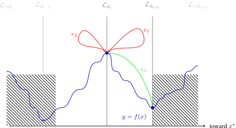
Figure 3: Illustration of a function f : {0, 1}n → R with a set of local maxima in layer Ldℓ where three kinds of excursions can occur: a failing left excursion in red, the right excursion that fails to reach Ldℓ+1 also in red and the successful one in green.
confined in the slope [dℓ+1, dℓ] where f is decreasing across the layers Ldℓ , . . ., Ldℓ+1 , our one-phase approximation in Lemma 6 applies once more and gives, here for OW, that an average number of O(1) right-excursions are needed in order to reach layer Ldℓ+1 and the total length of all these rightexcursions is O(n log(n)).
Moreover, upon leaving Ldℓ , there is a probability dℓ n (resp. n-dℓ n ) that the excursion will be a right-excursion (resp. leftexcursion) hence, the average number of left-excursions performed before a right-excursion occurs is n dℓ thus the average number of excursions needed is given by
using Wald's theorem [Wald, 1944] in the simplified version of [Doerr and K¨unnemann, 2015].
Finally, with Wald's theorem again and using the induction hypothesis on E[Tℓ], we obtain
since, for any i ∈ [1..k∗ ], we have
where the left-hand side does not depend on i. The stated result hence follows by considering the case ℓ = k + 1 in (1), where assumption k = O(1) implies that that the hidden constant in (1), which is a O(1)k , is still a O(1).
The factor O(n log(n)) in the complexity derived in Theorem 15 represents the expected time the MMAHH requires to transition from one local optimum to a neighboring local optimum. The other multiplicative factors, i.e., O(nk/(d1 · · · dk)), can be interpreted as the time needed for a biased random walk on the set of local optima, starting from (0, . . . , 0), to reach the global maximum.
The generality of our SEQOPT benchmark allows us to immediately extend our result in Theorem 15 to a variety of known benchmark functions, for which the MMAHH exhibits remarkable performance.
Corollary 16. Let p = Θ(1/n log(n)) and q = Θ(1/n log(n)). Then, the runtime T of the MMAHH
(i) on JUMPm with m ∈ [2.. n2 ] satisfies
(ii) on CLIFFd with d ∈ [2.. n2 ] satisfies
(iii) on CLIFFJUMPd,r,s with s ∈ N+, d, r ∈ [1.. n2 ] with r < d satisfies
These results highlight the power of MMAHH: on CLIFFd we incur only an extra O(logn) factor compared to the MAHH's O(n log n + n3 d2 ) runtime (using probability p = 1/((1+ε)n)) as stated in [Lissovoi et al., 2023], while achieving drastic speed-ups on JUMPm, reducing the O(n logn + n2m(1+ε)m-1 (m2 m!) ) bound of the MAHH, and similarly outperforming it on CLIFFJUMPd,r,s beyond the previously established O((d - r) (1+ε)r n2r+2 (r+1)2 (r+1)! ) result.
5 Conclusion
In this work, we proposed two new building-blocks for the design of efficient move-acceptance hyper-heuristics. The Markov chain-based selection of the acceptance operator instead of the random mixing strategy used in previous theoretical works already with non-elaborate switching probabilities like q = 1 2 greatly increases the rate of longer phases of the non-elitist selection operator (AM or OW), which led to provable significant speed-ups. The new OnlyWorsening (OW) acceptance operator was designed to aid the heuristic leave local optima. Used with the classic MAHH it gives comparable results as AM but, together with the Markov selection strategy it can lead to drastic speed-ups, e.g., polynomial runtimes on all SEQOPTk functions, k a constant. Both from the runtime guarantees proven in this work and from the working principles visible in our proofs we are very optimistic that our new building-blocks have a true potential for improving the hyper-heuristics used today.
The presented MMAHH algorithm mixing between OI and OW cannot traverse plateaus in the fitness landscape. The extension of these acceptance operators to accept solutions of equal fitness is an interesting direction for follow-up work. Furthermore, our theoretical analysis suggests that the empirical exploration of our proposed MMAHH is a promising direction for future research.
Acknowledgements
The research of B. Doerr is supported by the FMJH Program PGMO. J. Lutzeyer is supported by the French National Research Agency (ANR) via the "GraspGNNs" JCJC grant (ANR-24-CE23-3888).
@inproceedings{ijcai2025p984,
  title     = {Speeding Up Hyper-Heuristics With Markov-Chain Operator Selection and the Only-Worsening Acceptance Operator},
  author    = {Bendahi, Abderrahim and Doerr, Benjamin and Fradin, Adrien and Lutzeyer, Johannes F.},
  booktitle = {Proceedings of the Thirty-Fourth International Joint Conference on
               Artificial Intelligence, {IJCAI-25}},
  publisher = {International Joint Conferences on Artificial Intelligence Organization},
  editor    = {James Kwok},
  pages     = {8850--8857},
  year      = {2025},
  month     = {8},
  note      = {Main Track},
  doi       = {10.24963/ijcai.2025/984},
  url       = {https://doi.org/10.24963/ijcai.2025/984},
}
TY - CPAPER TI - Speeding Up Hyper-Heuristics With Markov-Chain Operator Selection and the Only-Worsening Acceptance Operator AU - Bendahi, Abderrahim AU - Doerr, Benjamin AU - Fradin, Adrien AU - Lutzeyer, Johannes F. T2 - Proceedings of the Thirty-Fourth International Joint Conference on Artificial Intelligence, IJCAI-25 PB - International Joint Conferences on Artificial Intelligence Organization PY - 2025 SP - 8850 EP - 8857 DO - 10.24963/ijcai.2025/984 UR - https://doi.org/10.24963/ijcai.2025/984 ER -Copied
Machine-readable versions of this paper, for tools and AI agents:





